Establishment and validation of an artificial intelligence-based model for real-time detection and classification of colorectal adenoma

Dataset and preprocessing

Colonoscopy images were obtained from the Digestive Disease Center of Beijing Hospital of Traditional Chinese Medicine, Capital Medical University using an EVIS LUCERA CF-HQ290I endoscopy system (Olympus Optical Co, Ltd.) Polyp images were subjected to binary classification and separated into two groups containing either all clinically classified adenomas or other types of polyps, including hyperplastic and inflammatory polyp, etc. Our rationale for using binary classification was based on two factors. First, from a pathological perspective, since adenoma is a high-risk factor for CRC, our main goal was to distinguish adenomas from other types of polyps. Second, our previous model showed that multi-classification of polyps reduced sensitivity. The specific reasons and visualization results can be viewed in Supplementary Fig. S1.

The entire datasets were captured and labeled by endoscopist blinded to the subjects, which contains 1436 images and 25 videos. We divide all image datasets into training, validation, and test sets. The test set accounts for one fifth of all images, with the remaining images divided into a ratio of 9:1 for training and testing sets. Images were categorized into white light imaging (WLI) and narrow band imaging (NBI) depending on the lens type, with a resolution of 566 × 478. Videos were obtained by NBI imaging with a resolution of 720 × 576, and 50.04 frames per second. All datasets were preprocessed identically before being passed to the model. First, we scaled the images to a fixed size of 416 × 416. Then, normalization of the whole image was performed. These operations were performed automatically before the picture was passed into the model, thereby allowing application of the same model to data from different sources without further adjustment. Several raw colonoscopy images from the dataset are shown in Supplementary Fig. S2.

Adaptive lightweight YOLOv4

The YOLOv4 model was proposed by Alexey et al. Similar to the YOLO family, the YOLOv4 algorithm innovatively treats object recognition as a regression problem, focusing on the probability of each object appearing in segmentation frames within an image. YOLOv4’s output includes the probability, center coordinates, and box size for each detected object. Because the entire detection pipeline comprises a single network, it allows for the direct end-to-end optimization of detection performance. Compared to two-stage object detection algorithms, optimizing the network structure is more straightforward with YOLOv4. The design of YOLO achieves efficient object detection, offering a new paradigm for single-stage object detection methodologies. Although single-stage detection is faster, it may exhibit a slight decrease in accuracy.

The real-time application success of the YOLOv4 model has been enhanced by the improvement of several YOLOv4 algorithms that have reduced the computational cost, improved the accuracy, and reduced the inference time²⁴. Compared with previous one-stage networks, YOLOv4 achieves a balance between speed and precision. However, adjusting the YOLOv4 backbone network and increasing or decreasing the number of convolutional layers only serves to improve the predictive ability of a specific dataset²⁵. In addition, the inference time of the model is constrained by the number of parameters and device memory. Thus, based on the structure of the YOLOv4 network, we have proposed a strategy that reduces the number of parameters without reducing the network accuracy.

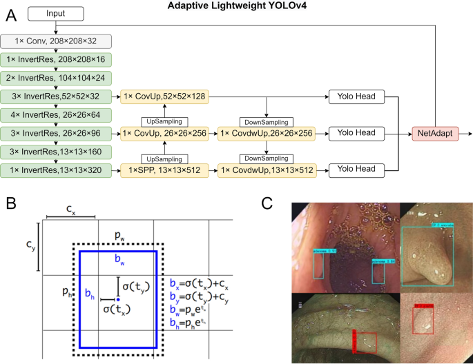
We utilized depthwise separable convolutions to reduce the number of standard convolutions. Unlike standard convolutions, depthwise separable convolutions operate in two steps. In the first step, a 3 × 3 convolution with a depth of one was applied to each channel of the input feature map. We regarded the output feature map as a whole, and the following convolutions were operated on the whole. Next, a 1 × 1 convolution was performed on the feature map with a convolution kernel equal to the number of output channels, and a convolution kernel depth equal to the input feature map²⁶. The application of depthwise separable convolutions reduced the required parameters of the original convolutions by more than eight times, with only a slight decrease in accuracy. From the lightweight perspective of the model, we replaced all 3 × 3 standard convolutions in the backbone network and path aggregation network (PANet) with depthwise separable convolutions. Next, we replaced the path aggregation network (CSPNet) structure in the backbone network with an inverted residual structure. Inverted residuals divide the input feature map into two branches. One branch generates convolution layers on the input, then directly stacks it with the other branch. Inverted residuals are different from the residual network of CSPNet, and multiply the input feature map. The expansion factor determines the degree of feature map extraction. Here, we adopted the same parameter settings described in the MobileNetv2 convolutional neural network, which were our requirements for model stability. The convolution layers of inverted residuals were replaced by depthwise separable convolutions. Next, the same value as the expansion factor was used for dimensionality reduction. Finally, the manipulated branch was stacked with the branch representing the residual. The improved structure enriches the gradient information in the network output. The input and output of the inverted residual structure are referred to as bottlenecks. Since the internal convolutions are one-time tensors, then the total memory occupied by the network training is only determined by the bottleneck. We chose this structure to improve memory efficiency while slightly improving accuracy.

Restricting the upper boundary of the activation function allows the network to have good numerical resolution even when the accuracy of mobile devices is low. We replaced the unbounded Mish activation function adopted by YOLOv4 backbone with ReLU6 activation function. In addition, we removed the last activation function of the inverted residual body. Previous studies have shown that ReLU6 activation after depthwise separable convolution operation results in information loss²⁷.

NetAdapt is an automated approach to network optimization that progressively reduces the resource consumption of pre-trained networks while ensuring maximum accuracy²⁸. A key advantage of using NetAdapt is that it can automatically pre-train deep neural networks for mobile platforms, depending on different resource budgets. NetAdapt constructs a hierarchical lookup table and measures the resource consumption of each layer in advance to determine the number of convolutional kernels and channels reserved in a given resource-constrained layer.

Our work significantly enhances YOLOv4’s efficiency for real-time detection by firstly employing depthwise separable convolutions, reducing computational load while maintaining accuracy. Secondly, we optimized the model’s structure with an inverted residual mechanism, improving memory efficiency and gradient richness. Thirdly, we adopted the ReLU6 activation function for better performance on low-precision devices. Finally, we utilized NetAdapt for automated, resource-aware network optimization, ensuring optimal accuracy within resource constraints. These innovations collectively streamline YOLOv4 for practical, efficient, and accurate real-time applications.

Single shot multibox detector (SSD)

Single shot multibox detector (SSD) is a popular and powerful target detection network²⁹. We applied VGG-16 in the initial basic network to improve the performance of predicting polyps smaller than 5 mm. The SSD model encapsulates localization and detection in the forward operation of the network, thereby significantly improving the training speed of the network.

VGG-16 serves as the backbone network in the single shot multibox detector (SSD) model, playing a crucial role in feature extraction for efficient object detection. As the backbone, VGG-16 is responsible for processing input images and extracting hierarchical features of varying scales. The network’s deep architecture, consisting of 13 convolutional layers with small 3 × 3 kernels, allows it to capture intricate details in the input images. In the context of SSD, these features are essential for detecting objects of different sizes. The uniformity of VGG-16’s structure aids in the extraction of high-level semantic information, contributing to a more robust representation of the input scene. The features obtained from VGG-16 are then used in multiple layers of the SSD model to generate predictions for object classes and bounding box coordinates. This integration leverages the strengths of VGG-16, facilitating accurate and efficient object detection across various scales within a single pass.

Ensemble learning

In clinical practice, most colorectal polyps are less than 5 mm. When small polyps are not detected and magnified during colonoscopy, the possibility of missed diagnosis increases. Such issues may be addressed through the development of models that improve the ability to detect small polyps, for example, by drawing prediction boxes as soon as the camera “flies by”. Ensemble learning allows both the lightweight network and small object detection ability to be taken into account³⁰.

The single shot multibox detector (SSD) excels at detecting small objects, largely thanks to its data processing and transformation capabilities. Considering its rapid detection and deep feature extraction abilities, we integrated these strengths with those of the adaptive lightweight YOLOv4 to mitigate its minor shortcomings, achieving a balance between training speed and accuracy. For ease of understanding, we have named this integrated model the adaptive small object detection ensemble model (ASODE model).

The ASODE model was trained by the AdaBoost algorithm, then the model predictions were combined using the soft voting method. Soft voting enhances the accuracy and robustness of the ASODE model by assigning greater weight to more reliable models, thus leveraging the collective information from multiple models to improve overall performance and generalization capability. It ensures the integration of predictions from multiple base models based on the probability or confidence scores for each class, guaranteeing that the final prediction takes into account the confidence level of each model.

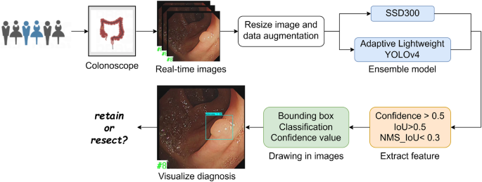
The architectural framework of our model segment has been meticulously crafted, marking a pivotal juncture where we transition to delineate the comprehensive operational methodology of the model, as illustrated in Fig. 1.

Initially, in pursuit of constructing a robust dataset, we embarked on collecting authentic colonoscopy imagery from patients potentially afflicted with colorectal polyps. This raw data underwent a rigorous process of scaling and augmentation, ensuring a rich dataset poised for deep learning.

Subsequently, these processed images are introduced into the ASODE model, a sophisticated amalgamation of adaptive lightweight YOLOv4 and SSD, designed for optimal efficiency and accuracy. The detailed structure of Adaptive lightweight YOLOv4 is shown in Fig. 2A. To refine the model’s discernment capabilities further, the images undergo a deep learning training phase. This phase leverages three stringent feature extraction thresholds to ensure the preservation of only the most relevant prediction boxes, thereby filtering out any potentially misleading data.

Example of the model training process. (A) Adaptive lightweight YOLOv4. (B) Parameters meaning and location of a bounding box. (C) Example of data augmentation.

Ultimately, the process generates a prediction box for each target, each meticulously classified and assigned a probability score. These are then seamlessly superimposed onto the original images, providing an intuitive visual representation of the model’s inferences. This end-to-end methodology not only epitomizes the cutting-edge in AI-driven diagnostic tools but also significantly enhances the interpretability and applicability of our model in real-world clinical settings.

Training techniques

In the polyp detection system, input images were divided into an \(S\times S\) grid. If the center of the bounding box for a detected object fell into a grid cell, then that grid cell was responsible for calculating the classification confidence and predicting the bounding boxes. Define \(p\) indicates the polyp that appears in the detection box. \(Pr\left(p\right)\) represents the probability that a polyp of a specific category exists within the predicted bounding box. \({IoU}_{pred}^{truth}\) represents the Intersection over Union (IoU) between the predicted box and the ground truth box. Therefore, the \(confidence(p)\) on the left side of the equation takes into account both the classification probability of polyps and the accuracy of the corresponding bounding box, and the product of the two is the confidence in predicting the existence of a certain type of polyps in the bounding box. The confidence of an object in the bounding box correspond to:

where \(B\) is the predicted box and \({B}^{gt}\) is the target box. If no polyps were present in the predicted box, then \(Pr\left(p\right)\) should be zero. Otherwise, the confidence scores were equal to the intersection over union (\(IoU\)) between the predicted box and the target box according to (2). Bounding box predictions depended on 4 parameters, \({b}_{x}\), \({b}_{y}\), \({b}_{w}\), and \({b}_{h}\), which are defined in (3)–(6) below:

where \({b}_{x}\) and \({b}_{y}\) are the predicted center coordinates of the bounding box, \({b}_{w}\) and \({b}_{h}\) are the predicted width and height of the bounding box. Specifically, \({t}_{x}\) and \({t}_{y}\) are the network’s output predictions for the center of the bounding box relative to the grid cell. They are constrained between 0 and 1 after being processed through the sigmoid function \(\sigma \left(\cdot \right)\), ensuring that the center coordinates of the bounding box fall within the current cell. \({c}_{x}\) and \({c}_{y}\) are the top-left coordinates of the cell assigned to the current bounding box. \({t}_{w}\) and \({t}_{h}\) represents the network’s output predictions for the width and height of the bounding box in log scale. \({p}_{w}\) and \({p}_{h}\) are the preset anchor dimensions for width and height, used to scale the predicted bounding box based on the network’s output. Therefore, the actual width and height are calculated by exponentiating these values and multiplying by the corresponding anchor dimensions. This process adjusts the predicted width and height to match the scale of objects as they appear in the input images, allowing the model to predict bounding boxes that closely fit the objects’ actual sizes. Prediction of the polyp size and location of a bounding box are shown in Fig. 2B.

A non-maximal suppression (NMS) method was used to ensure that each object was surrounded by only one prediction box. The highest classification confidence was reserved for each predicted box containing polyps. YOLO defined a confidence threshold. If the \(IoU\) between two bounding boxes was greater than the threshold, then the lower confidence bounding box was eliminated. If the \(IoU\) between two bounding boxes was not greater than the threshold, then both bounding boxes were reserved. Thus, no redundant bounding boxes were reserved, and the final reserved bounding boxes were the predicted boxes.

At the end of the training process, a loss function was calculated to evaluate the predicted box. Most object detection algorithms use the \(IoU\) to determine the degree of overlap between the predicted box and the ground target box defined by (7). However, the bounding box regression function should consider three geometric factors: overlap area, center distance and aspect ratio. \(CIoU\) loss function takes into account these factors to produce a fast convergence rate, which is formulated by (8).

where \(\mathop{b}\limits^{\rightharpoonup}\) and \(\overset{\lower0.5em\hbox{$\smash{\scriptscriptstyle\rightharpoonup}$}}{{b^{gt} }}\) are the center points of the predicted box \(B\) and target box \({B}^{gt}\), \(\rho \left(\cdot \right)\) is the Euclidean distance and \(c\) is the diagonal distansce between the minimum closure regions of two boxes. A positive trade-off parameter is denoted by \(\alpha\), and \(v\) quantifies the aspect ratio consistency according to (9) and (10).

where \(w\) and \(h\) are the width and height of the predicted box, and \({w}^{gt}\) and \({h}^{gt}\) are the width and height of the target box.

Evaluation metrics

The generalization performance of the model was reflected in the task requirements. We used true positive (TP), false negative (FN), FP, and true negative (TN) metrics to evaluate the model and determine whether the predicted box falls on the polyps. Consequently, we employed metrics such as precision, recall, F1 score, mean average precision (mAP), and accuracy to delineate the model’s performance as outlined in Eqs. (11) through (15).

We also used the mean average precision (mAP) metric, which is commonly used in target detection. The mAP averages AP values across all categories as shown in Eq. (14). Therefore, the performance of the model can be measured by a single metric

where \(Q\) is the number of polyp classifications, and \(AveP\left({\text{q}}\right)\) is the average precision for a given query.

Finally, accuracy measures the proportion of correct polyp classifications over all ground truth (GT). Here, ground truth refers to total number of samples, providing a benchmark for evaluating model performance.

Data augmentation

We applied different data enhancement methods to the two sub-models in the ASODE model. Each training image is randomly sampled using a selected data augmentation method. Data augmentation simulated polyps that were not closely detected by the lens, images that were selected according to the overlap strategy, or a patch were randomly sampled from the training images. Our small dataset had a significant advantage after data enhancement, because introduction of this new “extended” data augmentation technique generated more training images.

For adaptive lightweight YOLOv4, the Mosaic data augmentation algorithm was used to enrich the detection dataset and increase the robustness ability of the model. In the training process, four images were randomly selected, flipped, scaled, and the color intensity was randomly changed. Finally, an augmented image was generated by distributing the images along the four corners. The robustness of the network was increased through the use of a random scaling operation, which added multiple small targets. In addition, the stitched images increased the batch size, and improved the efficiency of batch normalization. An example of data augmentation is shown in Fig. 2C. The images here represent the results identified after model training. The blue boxes indicate adenomas, while the red boxes denote other types of polyps.

For SSD, one of the three methods of data augmentation was selected for each training image sampled patches with a minimum overlap of 0.1, 0.3, 0.5, 0.7, or 0.9 between the sampled image and the target polyp, or randomly sampled patches. Data augmentation strategies have been shown to significantly improve performance, especially on small datasets like PASCAL VOC³⁰.

Training parameters

Training was divided into two phases: the freeze phase and the unfreeze phase. This setting reduces the memory consumption and helps to leave the local optimal solution. Adam, an adaptive learning rate optimization algorithm designed specifically for training deep neural networks, was used in our model. Unlike the stochastic gradient descent (SDG), which may be trapped in the local optimal solution during training, Adam introduces the first-order momentum and second-order momentum, respectively, such that the adaptive learning rate can improve the optimization efficiency. Although Adam can fail to converge due to too small a learning rate in later iterations, this did not occur in our study. Here, the momentum was set at 0.9, and weight decay was set at 0.0005, while other parameters were used as previously described in the YOLOv4 study²⁴. In the prediction process, we retained a predicted box with classification confidence and intersection over union (IoU) greater than 0.5, while the non-maximal suppression (NMS) value was 0.3. Sample sizes were not checked using power analysis because the present study did not report statistical analysis results for between- or within-group variables. The parameters of the model are shown in Supplementary Table S1.