A fully autonomous robotic ultrasound system for thyroid scanning

Human participants and safety
All experiments with human participants were performed with the approval of the Guangzhou First People’s Hospital Review Board (K-2021-131-04). Our researchers explained the entire process to all participants, and all participants signed an informed consent form. Furthermore, we obtained consent from participants confirming their understanding of the open access nature of this journal.
With the approval of the ethical review committee, we recruited of three distinct groups of participants. The participants were over 18 years old, and of both sexes. None of the participants had following cases: (1) neck trauma or failure to heal after surgery; (2) inability to maintain a stable head position;(3) history of US gel allergies; (4) history of surgical resection of both thyroid lobes. The first group predominantly comprised college students, and we manually collected thyroid US data from 66 volunteers within this group using handheld US equipment. Simultaneously, we employed FARUS system to autonomously scan 70 volunteers (20–30 years of age, 19 females, 41 males), 13 of whom were scanned manually by 5 doctors. To address the limitations of handheld US equipment in accurately diagnosing nodules, we opted to employ portable US equipment to gather two additional sets of data. The second set of data was obtained from thyroid US scans of 29 middle-aged and elderly individuals within the community, chosen specifically to facilitate the training of the nodule segmentation network. Finally, the third group was composed of 19 patients (age 53.05 ± 5.90 years old, 12 females, 7 males) who underwent robotic thyroid scanning. This group played a pivotal role in verifying the diagnostic performance of our FARUS system. The recruitment bias primarily arises from the geographic scope of recruitment, limited to a specific region in China.
To ensure the safety of the participants, these five approaches were implemented in the FARUS system: (1) All the participants needed to complete an US gel allergy test before thyroid scanning. (2) The FARUS system used the UR3 collaborative robot, which will stop by itself in the event of a collision and a safety staff has been monitoring the operation of the robot arm. (3) We limited the working area of the robot arm (R < 45 cm), and once it crosses the working area, it will be forcibly stopped. (4) We set the contact force between 2.0 N and 4.0 N to ensure adequate contact with the skin and to prevent pressure-induced distortion of the thyroid anatomy. If the force exceeds 4.5 N, the robot will be automatically stopped. 5. The chair that participants used during scanning had wheels so that participants could move back if they felt uncomfortable.
Thyroid modeling
For the estimation of the thyroid scanning range, we obtained the head and neck CT images from the Southern Hospital of Southern Medical University. Those contrast-enhanced CT images were used to establish the 3D model of the thyroid. We selected 500 contrast-enhanced CT sequences from patients with thickness ranging from 0.625 mm to 0.9 mm for modeling. This included 250 male and 250 female patients, aged between 7 and 82. The CT images were acquired with Philips Gemini TF PET/CT scanner, and the resolution of the acquired DICOM data is 512 × 512. We used samples that represented all age group populations and covered people with body mass index (BMI) ranging from 17.1 to 27.8.
We defined 60 marker points to label the thyroid gland (see Fig. S1). They were 2 points above and below the isthmus of the thyroid; 8 points in the sagittal plane of the left and right lobes of the thyroid; and 2 points on the left and right of the entire thyroid cross-section; for the left and right lobes of the thyroid above the isthmus. The height is divided into five equal parts, and 4 points are marked on the upper, lower, left, and right sides of the 4 cross-sections, for a total of 32 points; After manually marking all the key points, our custom Python program will generate a 3D model and measure the average measurements of the various parts. Through this model, we obtained the morphological data of the thyroid. The average height of thyroid gland was 4.76 (±0.57) cm, and the average unilateral leaf width and thickness was 1.48 (±0.34) cm and 1.52 (±0.22) cm, respectively. Through regression analysis, we found that the width, length, thickness, and volume of the thyroid gland had very low correlations with gender, age, height, and weight. For this reason, the scan length was set to 6.47 cm based on the 3σ rule, and the scan width was set to 5.48 cm that was the probe width of 4.0 cm plus the average thyroid width.
Thyroid gland and nodule segmentation
We introduce a novel architecture called VariaNet, specifically designed for thyroid and nodule segmentation, as illustrated in Fig. 2a. The VariaNet architecture consists of two main models: the first model is responsible for thyroid gland segmentation, utilizing ResNet1848 as the encoder and UNet as the decoder. Our training dataset, SCUTG8K, is employed for training this model, using the dice loss as loss function. The second model, focused to nodule segmentation, uses ResNeXt 50 as the encoder and UNet as the decoder, integrating a custom loss function. Due to dataset variations from different US probes, the training process for thyroid nodule segmentation is divided into two stages. Initially, we use TN3K49 and our dataset, SCUTN10K, as the thyroid nodule image dataset for training the model. The second phase involves the application of transfer learning. During this phase, we use our dataset, SCUTN1K, which is generated using our specific probe, to train the thyroid nodule model.
To improve the segmentation performance of solid nodules, we introduce two tailor-made loss functions. Firstly, the feature loss function assigns higher weights to the isogenic part within the nodules’ area. This attention mechanism, represented by the Gaussian mask of the image, allows VariaNet to focus on the isogenic region within the nodule, consequently enhancing the segmentation results. The definition of the feature loss is as follows:
$${L}_{{{feat}}} =1-\frac{\widehat{{{pred}}} \, \cap \, {gt}}{\widehat{{{pred}}}\cup {gt}}\\ \,\widehat{{{pred}}} ={W}^{{{Gauss}}}\cdot {N}_{{{pred}}}\\ {W}^{{{Gauss}}} =1-{e}^{-\frac{{\left({gt}-{g}_{{{avg}}}\right)}^{2}}{2{{g}_{{{std}}}}^{2}}}$$
(1)
where \({N}_{{{pred}}}\) represent the prediction of the nodule mask, and \({gt}\) denote the ground truth of the nodule mask. The variables \({g}_{{{{avg}}}}\) and \({g}_{{{std}}}\) correspond to the mean and standard value, respectively, of the gland lobe intensity derived from the pseudo label, as illustrated in Fig. 2a. The second loss function used is called distance loss. The primary objective of this loss function is to assign increased weights to the false positives present in the model’s prediction mask. The Distance Loss is constructed based on a distance mask that is calculated using the distances to the pseudo gland label. It is defined as:
$$\,{L}_{{{dist}}}={W}^{{{dist}}}{\cdot G}_{{{pred}}}$$
(2)
$$\,{W}^{{{dist}}}=\left\{\begin{array}{cc}0 \hfill & p\in {G}_{{{pred}}}\\ {min} ({x}_{b,}{y}_b)\in {{Boundary}}\sqrt{{({x}_{p}-{x}_{b})}^{2}+{({y}_{p}-{y}_{b})}^{2}} & p \, \notin \, {G}_{{{pred}}}\end{array}\right.$$
(3)
where \({G}_{{{pred}}}\) represent the prediction of the gland mask, and \(\left({x}_{b},{y}_{b}\right)\) denote the boundary of the gland mask. The fundamental insight underlying this loss function is that the thyroid nodule mask must be spatially confined within or precisely aligned with the boundaries of the thyroid gland mask. Figure 2a shows feature loss presented by the gaussian mask, IoU loss and Distance Loss presented by Distance mask. By combining feature loss, distance loss and IoU loss, we develop iso-hybrid loss for segmentation in the three-level aspect echogenicity-, position- and map-level, which able to capture three aspects of segmentation. The iso-hybrid loss is defined as:
$$\,{L}_{{{IsoHy}}}=\,{L}_{{{iou}}}+\alpha {L}_{{{feat}}}+\beta {L}_{{{dist}}}$$
(4)
The framework is implemented using PyTorch 1.10.0 with CUDA 11.3 support. When the ImageNet pre-trained encoder is accessible, it is employed to initialize the model’s weights. During training, a batch size of 8 is utilized, and the ADAM optimizer is employed to optimize the model for a total of 40 epochs.
Scan planning
We used the Microsoft Azure Kinect DK depth camera to produce an initial scanning plan. We set up a Kinect camera at a distance of about 1.2 m from the seat, a height of about 1.5 m, and a 45° angle to the front of the seat. The camera acquisition parameters were set as: the color camera was set to a resolution of 1280 × 720, and the field of view was 90° × 59°; the depth camera was set to WFOV 2 × 2 binned, the resolution was 512 × 512, and the field of view was 120° × 120°; The frame rate was set to 30 FPS. We estimated the thyroid location using the neck and head skeleton joint points. Given variations in thyroid anatomy among populations, we introduced a process to locate the thyroid lobe. This involved utilizing ultrasound guidance and image segmentation for precise determination of its position.
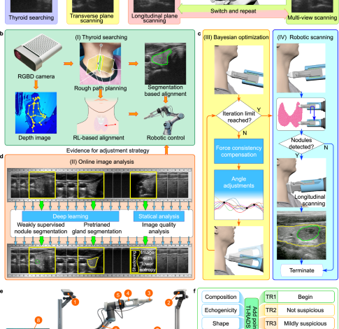
The robotic scanning involved switching between IPS and OPS phases, as mentioned in the “System design for autonomous ultrasound imaging” section. The IPS phase started with an optimized initial orientation achieved through Bayesian optimization. Inspired by the IPS procedure introduced in ref. 34, the probe then scanned upward and downward until both ends of the thyroid lobe were no longer visible in the segmentation image. During the IPS phase, VariaNet recorded suspicious nodule locations, guiding the subsequent OPS phase. To simulate doctors’ multi-view scanning, the OPS phase begins with a 60° probe rotation, followed by movement along the principal axis, covering a range of 12 mm. The image-based probe adjustment was achieved by calculating the intensity distribution of the US image as well as the center of mass in the segmentation mask, which enabled to prevent shadowing and keep the thyroid lobe in the center of the image.
Robotic scanning
The platform consisted of a UR3 robot that was a six-degree-of-freedom robotic arm with a repeatability of 0.1 mm, a working radius of 500 mm, and a maximum load of 3 kg. We used the real-time port for monitoring, which fed back the status of the robot arm at a speed of 125 Hz. For general robotic arm commands, such as motion commands, we sent them through the secondary port, which received commands at 10 Hz. Moreover, we used SolidWorks to design a fixture for the probe, which was 3D printed with photosensitive resin. To avoid excessive pressure on the participants, we attached the US probe to the robot flange with four flexible spring-loaded connection (Fig. S2). And the length of the entire robot end effector was 242 mm. We used a SonoStar C5 Laptop Color Doppler Ultrasound System. This US depth was between 18 mm and 184 mm, the US frequency range was 6.5 MHz to 10 MHz. The original US data had a resolution of 512 × 512 and were stored in the AVI format.
Prior to scanning, participants assumed a seated position on a chair and adjusted their posture. Subsequently, the Kinect camera captured a depth map, which was then employed to generate a 3D point cloud of the environment. This point cloud underwent analysis for real-time detection and tracking of the human body joints by the Kinect body-tracking algorithm50. Then the position of the thyroid was estimated based on spatial information derived from tracked human skeleton joints. The robot approaches the pre-estimated position at a speed of 10 mm/s. When the distance between the probe and participant is approximately less than 200 mm, the speed of robot end effector will be reduced to 5 mm/s. The FARUS started scanning procedure when the probe reaches the pre-determined position and the force is in the range of 2.0 N to 4.0 N. During the scanning process, the participant was allowed to move slightly and the robot was able to adapt to the participant’s movement through the force control and image servo. However, the scanning will be terminated if FARUS detects that the participant moves more than 2 cm left or right within 1 s, or 5 cm forward or backward. We chose the Robotiq FT300-S as the force/torque sensor. Its maximum range was \({{{{{{\bf{F}}}}}}}_{{{{{{\rm{x}}}}}}}={{{{{{\bf{F}}}}}}}_{{{{{{\rm{y}}}}}}}={{{{{{\bf{F}}}}}}}_{{{{{{\rm{z}}}}}}}=\pm 300\)N, and the sensor signal noise was 0.1 N. The control terminal read force information in real time at a speed of 100 Hz.
Control strategy
During robotic scanning, the control strategy we developed allows us to adjust the position and orientation of the probe autonomously. The US probe has a total of six degrees of freedom that can be adjusted. As illustrated in Fig. 5a, force control can be used to control one degree of freedom: the amount of translation of the robot in the \({{{{{{\bf{Y}}}}}}}_{{{{{{\rm{p}}}}}}}\) direction. The degree of freedom of US probe rotation around the \({{{{{{\bf{Y}}}}}}}_{{{{{{\rm{p}}}}}}}\) axis is controlled by switching between transverse and longitudinal views. Bayesian optimization is applied to control the rotational degrees of freedom of the probe around the \({{{{{{\bf{Z}}}}}}}_{{{{{{\rm{p}}}}}}}\) axis. The remaining three degrees of freedom are determined by the US image. Degrees of freedom in the \({{{{{{\bf{X}}}}}}}_{{{{{{\rm{p}}}}}}}\) axis and \({{{{{{\bf{Z}}}}}}}_{{{{{{\rm{p}}}}}}}\) axis translation of the US probe are controlled by the image segmentation results. While the degree of freedom of US probe rotation around the \({{{{{{\bf{X}}}}}}}_{{{{{{\rm{p}}}}}}}\) axis is controlled by image intensity distribution.
Keeping the contact force applied to the body under control is vital to the safety of the participants. The external forces \({{{{{\boldsymbol{f}}}}}}\) and torques \({{{{{\boldsymbol{\tau }}}}}}\) measured in the force sensor frame \({{{{{\mathcal{F}}}}}}\) is a 6-D vector \({{{{{\bf{H}}}}}}=({{{{{{\boldsymbol{f}}}}}}}^{T}{{{{{{\boldsymbol{\tau }}}}}}}^{T})\). The force/torque vector in the probe frame \({{{{{\mathcal{P}}}}}}\) can be written as:
$$\,{{\,\!}^{p}{{{{{\bf{H}}}}}}}_{p}=\,{{\,\!}^{p}{{{{{\bf{F}}}}}}}_{f}({{{{{\bf{H}}}}}}-{{\,\!}^{f}{{{{{\bf{F}}}}}}}_{g}{{\,\!}^{g}{{{{{\bf{H}}}}}}}_{g})$$
(5)
where \({\,\!}^{g}{{{{{\bf{H}}}}}}_{g}\in {{\mathbb{R}}}^{6}\) is the gravity force of the US probe, and represent the transformation matrix from frame \({{{{{\mathcal{F}}}}}}\) to frame \({{{{{\mathcal{P}}}}}}\) and the transformation matrix from the probe’s inertial frame to frame \({{{{{\mathcal{F}}}}}}\), respectively. Our objective is to control the force along the y-axis in the probe frame \({{{{{\mathcal{P}}}}}}\), we define the target contact force as:
$${{{{{{\rm{t}}}}}}}_{{{{{{\rm{f}}}}}}}={{{{{{\bf{S}}}}}}}_{{{{{{\rm{y}}}}}}}{{\,\!}^{{{{{{\rm{p}}}}}}}{{{{{\bf{H}}}}}}}_{{{{{{\rm{p}}}}}}}$$
(6)
where \({{{{{{\bf{S}}}}}}}_{{{{{{\rm{y}}}}}}}\) = (0 1 0 0 0 0). According to the visual servo control law \(\dot{s}={{{{{{\boldsymbol{L}}}}}}}_{s}{{{{{{\boldsymbol{v}}}}}}}_{c}\)51, the control law for the force control task is given by:
$$\,{v}_{f}=-\frac{{\lambda }_{f}}{k}({{{{{{\boldsymbol{S}}}}}}}_{y}{{\,\!}^{p}{{{{{\bf{F}}}}}}}_{f}({{{{{\bf{H}}}}}}-{{\,\!}^{f}{{{{{\bf{F}}}}}}}_{g}{{\,\!}^{g}{{{{{\bf{H}}}}}}}_{g})-{t}_{f}^{*}){{{{{{\boldsymbol{S}}}}}}}_{y}^{T}$$
(7)
where \({\lambda }_{f}\) is the force control gain, \({t}_{f}^{*}\) is the desired force value and k is the human tissues stiffness that is usually set in [125, 500] N/m according to ref. 52.
The sweeping trajectory T is defined by N waypoints \(\left\{{w}_{0},{w}_{1},\ldots,{w}_{n}\right\}\) and a speed v to travel along the trajectory. The waypoint \({w}_{0}\) is defined as the position where the probe orientation is optimized after Bayesian optimization procedure. In the case of scanning toward the upper or lower poles of the thyroid, the next waypoint \({w}_{i}\) would be a stride from the previous waypoint \({w}_{i-1}\). The position and orientation of the probe is adjusted after each step of movement by: (1) a translation along the \({{{{{{\bf{Y}}}}}}}_{{{{{{\rm{p}}}}}}}\) axis to achieve sufficient contact between the probe and the neck. (2) a translation along the \({{{{{{\bf{Z}}}}}}}_{{{{{{\rm{p}}}}}}}\) axis to ensure that the segmented thyroid is located in the center of US image. (3) A sideway correction to avoid the shadowing. Similar to ref. 34, the image-based sideway correction is carried out in an iterative manner:
$$\,{{{{{{\bf{R}}}}}}}_{{{{{{\rm{step}}}}}}}=\,\left[\begin{array}{ccc}1 & 0 & 0\\ 0 & cos ({\theta }_{{step}}) & -sin ({\theta }_{{step}})\\ 0 & sin ({\theta }_{{step}}) & cos ({\theta }_{{step}})\end{array}\right]$$
(8)
$$\,{{{{{{\bf{R}}}}}}}_{n}={{{{{{\bf{R}}}}}}}_{{step}}\cdot {{{{{{\bf{R}}}}}}}_{n-1}$$
(9)
where \({{{{{{\bf{R}}}}}}}_{{step}}\) is the rotation matrix defined by the rotation adjustment step of \({\theta }_{{step}}\) in the \({{{{{{\bf{Y}}}}}}}_{{{{{{\rm{p}}}}}}}\)–\({{{{{{\bf{Z}}}}}}}_{{{{{{\rm{p}}}}}}}\) plane, \({{{{{{\bf{R}}}}}}}_{n}\) represents the probe orientation after n adjustments.
Thyroid nodules scoring and classification
The ACR TI-RADS is a risk stratification system designed to help radiologists categorize thyroid nodules based on their US characteristics47. It provides a standardized way to assess the risk of malignancy for thyroid nodules, which can then guide the management and follow-up recommendations for patients. Figure 6b illustrates a sample outcome obtained from the ACR-TIRADS calculation:
-
(1)
Echogenicity, composition and echogenic foci: to assess the echogenicity, composition, and echogenic foci of the thyroid nodule, we analyze the distribution of pixels in the thyroid gland and the nodule, as depicted in Fig. 6c. Initially, we create a smooth line graph representing the pixel distribution in the thyroid gland and calculate the line average of the number of pixels. By selecting thyroid gland pixels above this line average, we determine the mean and standard deviation. Using the same method, we identify thyroid nodule pixels and calculate the percentage of echogenicity, composition, and presence of echogenic foci based on specific boundaries, such as cystic, hypo-genicity, iso-genicity, hyper-genicity, and calcification.
-
(2)
Margin and shape: the determination of the thyroid nodule’s margin involves two factors. Firstly, we consider the boundary line of the nodule, assessing distinctive pixels on its outer and inner edges. This factor is calculated by determining the mean standard deviation of 10 perpendicular pixels along each pixel of the nodule’s boundary line (5 inner pixels + 1 mid pixel + 5 outer pixels). Secondly, we analyze the shape of the boundary line by calculating the intersection over union (IoU) between the nodule and the fitted ellipse. The aspect ratio is another important shape characteristic, indicating the ratio of depth to width and revealing whether the nodule appears taller-than-wide. This aspect ratio provides valuable insight into the tumor’s growth pattern and is associated with an elevated risk of malignancy if it is higher.
Statistics and reproducibility
No statistical method was used to predetermine sample size. To assess the robotic image quality of US scans, we employed the FARUS system to autonomously scan 70 college students (n = 70). Additionally, to investigate the diagnostic performance of our FARUS system, robotic thyroid scanning was performed on 19 patients (n = 19). Overall, the robotic thyroid scans were successfully performed on 89 participants. Additionally, a transparent reporting of a multivariable prediction model for individual prognosis or diagnosis (TRIPOD) checklist is provided as Supplementary Table S3.
Reporting summary
Further information on research design is available in the Nature Portfolio Reporting Summary linked to this article.


