A sustainable and secure load management model for green cloud data centres

April 13, 2024

57 18 minutes read

Untitled design6 — 41598 2023 27703 Fig1 HTML.png

A Sustainable CDC infrastructure is organized utilizing P servers {$S_1$, $S_2$, …, $S_P$} located within n clusters {$CS_1$, $CS_2$, …, $CS_n$}, powered by Renewable Source of Energy (RSE) and grid via battery energy storage system as illustrated in Fig. 7. The electric power produced by multiple RSE such as solar panels, wind energy, and power grid charge battery storage including Uninterruptible Power Supply (UPS) which is discharged to provide required power supply and backup to clusters of servers {$CS_1$, $CS_2$, …, $CS_n$}. Consider M users {$U_1$, $U_2$, …, $U_M$} submit job requests {$\lambda _1$, $\lambda _2$, …, $\lambda _M$} for execution on their purchased VMs {$V_1$, $V_2$, …, $V_Q$}$: M<Q$, where Q is a total number of available VMs and one job may execute on multiple VMs.

A Resource Management Unit (RMU) is set up to receive and distribute these requests among VMs deployed on servers {$S_1$, $S_2$, …, $S_P$}. RMU is employed to acquiesce secure and energy-efficient resource distribution based load balancing for sustainability and security augmentation within CDC. Further, it controls all the privileges of physical resource management such as handling of over-/under-loading of servers, VM placement, VM migration, scheduling etc. RMU is obliged for two-phase scheduling including (i) distribution of job requests {$\lambda _1$, $\lambda _2$, …, $\lambda _M$} among VMs and (ii) placement of VMs {$V_1$, $V_2$, …, $V_Q$} on servers. Accordingly, it assigns job requests {$\lambda _1$, $\lambda _2$, …, $\lambda _M$} among VMs corresponding to the user specified resource (viz., CPU, memory, bandwidth) capacity. Further, it appoints a multi-objective load balancing optimization for allocation of users’ VMs {$V_1$, $V_2$, …, $V_Q$} to available physical servers {$S_1$, $S_2$, …, $S_P$} subject to security and energy-efficiency.

A Cloud Workload and Resource Usage Analyser (CW-RUA) is employed to estimate the workload and physical resource usage proactively and assist RMU by providing useful knowledge of resource provisioning in anticipation. CW-RUA captures the historical and live traces of resource utilization by VMs {$V_1$, $V_2$, …, $V_Q$} hosted on different servers {$S_1$, $S_2$, …, $S_P$} within clusters {$CS_1$, $CS_2$, …, $CS_n$}. The workload and resource usage analysis is performed in two steps: (i) Data preparation and (ii) Predictor optimization which are executed periodically. Data is prepared in the form of a vector of learning window using three consecutive steps including aggregation of resource usage traces, rescaling of aggregated values, followed by normalization. The learning window vector is passed to a neural network-based predictor which is trained/optimized with the help of a novel DPBHO evolutionary optimization algorithm. The detailed description of DPBHO, CW-RUA and Secure and Sustainable VMP (SS-VMP) is elucidated in Sections “Dual-phase black-hole optimization”, “Cloud workload resource usage analysis” and “Secure and sustainable VM placement”, respectively.

Dual-phase black-hole optimization

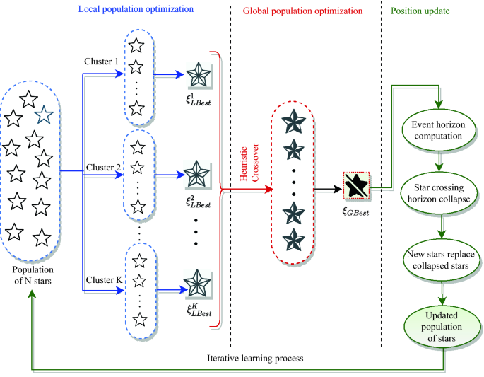
A two-phase population-based optimization algorithm named Dual Phase Black-Hole Optimization (DPBHO) is proposed, wherein each phase, the candidate solutions are considered as stars while a star with the best fitness value is observed as a black-hole. Figure 8 portrays the DPBHO design which incorporates three consecutive steps: (i) Local population optimization, (ii) Global population optimization, and (iii) Position Update.

Local population optimization

In this phase, the stars i.e., random solutions {$\xi _1$, $\xi _2$, …, $\xi _\mathbb {N}$}$\in \mathbb {E}$ are organized into K clusters or sub-populations, each of size $\mathbb {N}/K$. All the members of each cluster ($\xi _i^k: i \in [1, \mathbb {N}/K], k \in [1, K]$) are evaluated over training data using fitness value ($f_i^k$) obtained by computing Eq. (1), where $F(\xi _i^k)$ is a fitness evaluation function. The best solution of each $k^{th}$ cluster is considered as its local blackhole ($\xi ^{k}_{Lbest}$) such that $\xi ^{k}_{Lbest} =$ Best({$\xi _1$, $\xi _2$, …, $\xi _{\mathbb {N}/K}$}).

$$\begin{aligned} f_i^k = F(\xi _i^k) \quad \forall i \in [1, \mathbb {N}/K], k \in [1, K] \end{aligned}$$

(1)

Global population optimization

In the global optimization phase, all the local blackholes consitute the second phase population {$\xi ^{1}_{Lbest}$, $\xi ^{2}_{Lbest}$, …, $\xi ^{K}_{Lbest}$}, wherein heuristic crossover is performed to raise diversity of the second phase population by producing new individuals with a superior breed. In the course of heuristic crossover, stars act as chromosomes, where two parent chromosomes are randomly chosen and their fitness values are compared to find out the parent with better fitness value. Afterward, a new offspring is produced with the combination of two parent chromosomes using Eq. (2) which is closer to the parent having better fitness value²⁴. This additional step brings significant diversity in the search space by adding new and better individuals in the second phase population. Let $\xi ^{k}_{Lbest}$ and $\xi ^{j}_{Lbest}$ be two parent chromosomes, wherein $\xi ^{k}_{Lbest}$ is considered as a parent chromosome with better fitness value. Thereafter, the offspring $\xi _{Off}$ is generated as follows:

$$\begin{aligned} \xi _{Off} = Cr_i(\xi ^{k}_{Lbest_i}-\xi ^{j}_{Lbest_i}) + \xi ^{k}_{Lbest_i} \quad i \in [1, L] \end{aligned}$$

(2)

where, $Cr_i$ is a randomly generated crossover rate in the range [0, 1] for $i^{th}$ gene such that i =$\{1,2, \ldots , L\}$, $\xi _{Off}$ is new offspring, $\xi ^{k}_{Lbest_i}$ and $\xi ^{j}_{Lbest_i}$ are $i^{th}$ gene of parents: $\xi ^{k}_{Lbest}$ and $\xi ^{j}_{Lbest}$, respectively such that $k \ne j$. A new offspring is produced for each of K (which is equals to the total number of local blackholes) heuristic crossover. Equation (3) is applied to select best between new offspring ($\xi _{Off}$) and parent with lesser fitness ($\xi ^{j}_{Lbest}$). This allows to enhance the diversity of the local population with members of enriched fitness value.

$$\begin{aligned} \xi ^{j}_{Lbest}={\left\{ \begin{array}{ll} \xi _{Off} &{} \text {If (fitness}(\xi _{Off}) \ge {\hbox {fitness}} (\xi ^{j}_{Lbest})) \\ \xi ^{j}_{Lbest} &{} {\text {Otherwise}} \end{array}\right. } \end{aligned}$$

(3)

Thereafter, a best among the members of second phase population is nominated as global blackhole ($\xi ^{k}_{Gbest}$).

Position update

The position of stars is updated in accordance with $\xi ^{k}_{Lbest}$ and $\xi ^{k}_{Gbest}$ as depicted in Eq. (4), where $\xi _i^k(t)$ and $\xi _i^k(t+1)$ are the positions of $i$th star of $k$th sub population at time instances t and $t+1$, respectively. $r_1$ and $r_2$ are random numbers in the range (0, 1) while $\alpha _l$ and $\alpha _g$ are the attraction forces applied on $\xi _i^k(t)$ by $\xi ^{k}_{Lbest}$ and $\xi ^{k}_{Gbest}$, respectively. The inclusion of local best in position update procedure maintains the diversity of stars by gradually controlling the convergence speed and retains their exploratory behaviour.

$$\begin{aligned} Lf(t)= \alpha _1^k r_1\big (\xi ^{k}_{Lbest}(t)-\xi _i^k(t) \big )\\ Gf(t)= \alpha _gr_2\big (\xi ^{k}_{Gbest}(t) – \xi _i^k(t)\big ) \\ \xi _i^k(t+1)= \xi _i^k(t)+Lf(t) +Gf(t) \end{aligned}$$

(4)

The fitness value of all the updated stars is computed by applying Eq. (1). In case, if kth cluster locates a better solution than the existing one, the respective $\xi ^{k}_{Lbest}$ is replaced and $\xi ^{k}_{Gbest}$ is updated as per the admissibility. SB algorithm is inspired by the natural blackhole phenomenon, where a blackhole consumes everything that enters it including light. DPBHO algorithm works on the concept of a standard blackhole optimization algorithm, wherein none of the candidate solutions is allowed to return from an event horizon (h) area of a blackhole solution delineated by its radius ($\mathbb {R}_h$). The ratio between fitness value of a local blackhole ($f(\xi ^{k}_{Lbest})$) and fitness value of its sub-population ($\sum _{i=1}^{\mathbb {N}/K}{f(\xi ^{k}_{i})}$) computes the event horizon radius ($\mathbb {R}_h\big (\xi ^{k}_{Lbest}\big )$) of the respective blackhole as given in Eq. (5). Similarly, the event horizon radius of a global blackhole ($\mathbb {R}_h\big (\xi ^{k}_{Gbest}\big )$) is evaluated using Eq. (6), where $f(\xi ^{k}_{Gbest})$ is fitness value of global blackhole, $\sum _{k=1}^{K}\sum _{i=1}^{\mathbb {N}/K}{f(\xi ^{k}_{i})}$ is a fitness value of the entire population.

$$\begin{aligned}{} & {} \mathbb {R}_h\big (\xi ^{k}_{Lbest}\big )=\frac{f(\xi ^{k}_{Lbest})}{\sum _{i=1}^{\mathbb {N}/K}{f(\xi ^{k}_{i})}} \quad k \in [1, K] \end{aligned}$$

(5)

$$\begin{aligned}{} & {} \quad \mathbb {R}_h\big (\xi ^{k}_{Gbest}\big )=\frac{f(\xi ^{k}_{Gbest})}{\sum _{k=1}^{K}\sum _{i=1}^{\mathbb {N}/K}{f(\xi ^{k}_{i})}} \end{aligned}$$

(6)

The distance between both solutions is estimated by utilizing the arithmetic difference of their fitness values to confirm that a member solution has reached into the event horizon of the blackhole solution. The distance from local and global blackholes is calculated because each solution gets attracted to these two blackholes. Accordingly, the distance of ith star ($\xi ^{k}_{i}$) of kth sub-population from local blackhole ($\xi ^{k}_{Lbest}$) and global blackhole is computed in Eqs. (7) and (8), respectively.

$$\begin{aligned}{} & {} \mathbb {D}_{\xi ^{k}_{Lbest}}\big (\xi ^{k}_{i}\big )=f(\xi ^{k}_{Lbest}) – f(\xi ^{k}_{i}) \quad i \in [1, \mathbb {N}/K] \end{aligned}$$

(7)

$$\begin{aligned}{} & {} \quad \mathbb {D}_{\xi ^{k}_{Gbest}}\big (\xi ^{k}_{i}\big )=f(\xi ^{k}_{Gbest}) – f(\xi ^{k}_{i}) \quad i \in [1, 2K] \end{aligned}$$

(8)

If the distance between candidate solution $\xi ^{k}_{i}$ and local blackhole ($\xi ^{k}_{Lbest}$) is less than or equals to the event horizon radius of $\xi ^{k}_{i}$ i.e., $\mathbb {R}_h\big (\xi ^{k}_{Lbest}\big )$ then $\xi ^{k}_{i}$ gets collapse which is replaced by a new randomly generated solution to keep uniform number of solutions throughout the simulation. Following the same procedure, $\xi ^{k}_{i}$ gets collapse and replaced by a new random solution when it enters into the event horizon radius of the global blackhole $\mathbb {R}_h\big (\xi ^{k}_{Gbest}\big )$. The operational summary of DPBHO is given in Algorithm 1.

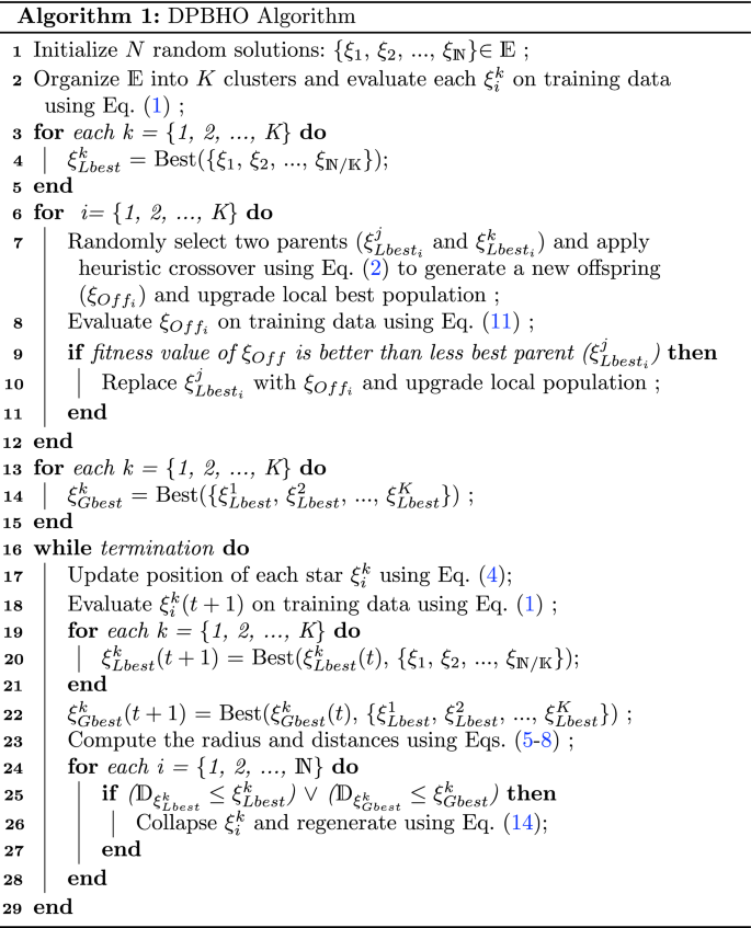
Step 1 initializes random solutions, and has complexity $\mathcal {O}(1)$. Step 2 evaluates the fitness of $\mathbb {N}$ solutions with $\mathcal {O}(\mathbb {N})$ complexity. Steps [3–5], steps [6–12], and steps [13–15] iterate K times and have equal time complexity of $\mathcal {O}(K)$. Assume steps [16–29] repeat for t intervals, wherein steps [19–21] have $\mathcal {O}(K)$ while steps [24–28] have $\mathcal {O}(\mathbb {N})$ complexities. Hence, the total time complexity for the DPBHO algorithm is $\mathcal {O}(\mathbb {N}Kt)$.

An illustration

Let there are 9 solutions (or stars) in the initial population ($E^1$) as shown in Table 9 which are grouped into 3 clusters during the first generation or epoch such that $Cluster_1^1$ (Table 10), $Cluster_2^1$ (Table 11), and $Cluster_3^1$ (Table 12). The fitness of each candidate solution is estimated using Eq. (11) and local best candidate is selected from each cluster. Likewise, $\xi _{Lbest_1}$, $\xi _{Lbest_2}$, and $\xi _{Lbest_3}$ constitute local best population (Table 13). The heuristic crossover operation is performed to improve the local best population using Eq. (2) and a global best candidate ($\xi _{Gbest}$) is chosen after fitness evaluation as depicted in Table 14. Further, the population is updated by computing event horizon radius for each cluster as well as a global radius of entire population as observed in Table 15. The distance of each candidate of the first generation population is estimated using Eqs. (7) and (8) to generate the next generation population as illustrated in Table 16, wherein the candidates $\xi _1$, $\xi _5$, $\xi _6$, and $\xi _8$, are updated.

Table 9 Initial generation population ($E^1$).

Table 10 (${Cluster^1_1}$).

Table 11 ${Cluster^1_2}$.

Table 12 ${Cluster^1_3}$.

Table 13 Local best population. ($\xi _{Lbest}^1$).

Table 14 Global best candidate ($\xi _{Gbest}^1$) after Heuristic Crossover.

Table 15 Event horizon computation.

Table 16 Second generation population ($E^2$).

Cloud workload resource usage analysis

The cloud workload analysis comprises of two steps: data preparation and multi-layered feed-forward neural network (MFNN) optimization using DPBHO algorithm as described in detail in the following subsections.

Data preparation

MFNN derives intial information for data preparation from Historical Resource Usage database of different clusters {$CS_1$, $CS_2$, …, $CS_n$} which is updated periodically with live resource usage information as portrayed in block CW-RUA of Fig. 7. Let the received historical resource usage information: {$d_1$, $d_2$ , …, $d_z$}: $\in \varpi ^{In}$ is aggregated with respect to a specific time-interval (for example, 1 min, 5 min, 10 min, 60 min and so on). The aggregated values have high variance which are rescaled within the range [0.001, 0.999] by applying Eq. (9), where $\varpi ^{In}_{min}$ and $\varpi ^{In}_{max}$ are the minimum and maximum values of the input data set, respectively. The normalized vector is denoted as $\hat{\varpi ^{In}}$, which is a set of all normalized input data values as $\hat{\varpi ^{In}}$.

$$\begin{aligned} \hat{\varpi ^{In}}= 0.001 +\frac{ d_i- \varpi ^{In}_{min}}{\varpi ^{In}_{max}-\varpi ^{In}_{min}}\times (0.999) \end{aligned}$$

(9)

These normalized values (in single dimension) are organized into two dimensional input and output matrices denoted as $\varpi ^{In}$ and $\varpi ^{Out}$, respectively as stated in Eq. (10):

$$\begin{aligned} \varpi ^{In}= \left[ {\begin{array}{cccc} \varpi _1 &{} \varpi _2 &{} …. &{} \varpi _z\\ \varpi _2 &{} \varpi _3 &{} …. &{} \varpi _{z+1} \\ . &{} . &{} …. &{} . \\ \varpi _m &{} \varpi _{m+1} &{} …. &{} \varpi _{z+m-1} \\ \end{array} } \right] \varpi ^{Out}= \left[ {\begin{array}{c} \varpi _{z+1} \\ \varpi _{z+2} \\ . \\ \varpi _{z+m} \end{array} } \right] \end{aligned}$$

(10)

MFNN optimization

The prepared data values $\varpi ^{In}$ are divided into three groups: training (60%), testing (20%), and validation (20%) data, where training data is used to optimize the predictor while testing data is used for evaluating the prediction accuracy over unseen data. During training, MFNN extracts intuitive patterns from actual workload ($\varpi ^{In}$) and analyzes z previous resource usage values to predict the $(z+1)$th instance of workload in each pass. In the course of training and testing period, the performance and accuracy of the proposed model is evaluated by estimating the Mean Squared Error ($\varpi ^{MSE}$) score as fitness function) using Eq. (11); where $\varpi ^{AO}$ and $\varpi ^{PO}$ are actual and predicted output, respectively²⁵. Further, validation data is applied to confirm the accuracy of the proposed prediction model, wherein Mean absolute error ($\varpi ^{MAE}$) stated in Eq. (12) is used as a fitness function because it is an easily interpretable and well established metric to evaluate regression models.

$$\begin{aligned} \varpi ^{MSE}= & {} \frac{1}{m}\sum _{i=1}^{m}(\varpi ^{AO}_{i}-\varpi ^{PO}_{i})^2 \end{aligned}$$

(11)

$$\begin{aligned} \varpi ^{MAE}= & {} \sum _{i=1}^{m}{\frac{\Vert \varpi ^{AO}_{i}-\varpi ^{PO}_{i}\Vert }{m}} \end{aligned}$$

(12)

In the proposed approach, MFNN represents a mapping p–$q_1$–$q_2$–$q_3$–r, wherein p, $q_1$, $q_2$, $q_3$ and r are the numbers of neurons in input, hidden$\#1$, hidden$\#2$, hidden$\#3$, and output layer, respectively. Since the output layer has only one neuron, the value of r is constantly 1. The activation function used to update a neuron is stated in Eq. (13), where a linear function ($(\varpi )$) is applied to input layer neurons and sigmoid function ($\frac{1}{1+e^{-\varpi }}$) for the rest of the neural layers.

$$\begin{aligned} f(\varpi )={\left\{ \begin{array}{ll} \varpi &{} \text {If (Input layer)} \\ \frac{1}{1+e^{-\varpi }} &{} {\text {otherwise.}} \end{array}\right. } \end{aligned}$$

(13)

The training begins with randomly generated $\mathbb {N}$ networks of real-numbered vectors denoted as {$\xi _1$, $\xi _2$, …, $\xi _\mathbb {N}$}$\in \mathbb {E}$, wherein each vector ($\xi _i: 1 \le i \le \mathbb {N}$) has size $L=$(($p+1$)$\times q_1+ q_1 \times q_2 +q_2 \times q_3 + q_3 \times r$). The number of neurons in input layer become $p+1$ by reason of consideration of one additional bias neuron. The synaptic or neural weights ($W^*_{ij}$) are generated randomly with uniform distribution as shown in Eq. (14), where $lb_j =-1$ and $ub_j =1$ are the lower and upper bounds, respectively and r is a random number in the range [0, 1].

$$\begin{aligned} W^*_{ij} = lb_j + r \times (ub_j – lb_j) \end{aligned}$$

(14)

MFNN is optimized periodically using DPBHO by considering each network vector ($\xi _i: 1 \le i \le \mathbb {N}$) as a star, where Eq. (11) is applied as a fitness function and the candidate having least fitness value is nominated as a best candidate both in local and global population optimization phase.

Secure and sustainable VM placement

Let $\omega$ represents a mapping between VMs and servers such that $\omega _{kji}=1$, if server $S_i$ hosts $V_j$ of $k^{th}$ user, else it is 0 as stated in Eq. (15).

$$\begin{aligned} \omega _{kji}={\left\{ \begin{array}{ll} 1 &{} \text {If (VM }V_j \text { of } k\text {th user is hosted on server }S_i) \\ 0 &{} {\text {Otherwise.}} \end{array}\right. } \end{aligned}$$

(15)

The essential set of constraints that must be satisfied concurrently have been formulated in Eq. (16):

$$\begin{aligned} \left. \begin{array}{ll} C_1: \quad \sum _{k \in M}\sum _{j \in Q}\sum _{i \in P}{\omega _{kji}}=1\\ C_2: \quad \sum _{k \in M} \sum _{j \in Q}\sum _{i \in P}{V_j^{C}} \times \omega _{kji} \le S_i^{C^{*}}\\ C_3: \quad \sum _{k \in M}\sum _{j \in Q}\sum _{i \in P}{V_j^{M}} \times \omega _{kji} \le S_i^{M^{*}}\\ C_4: \quad \sum _{k \in BW}\sum _{j \in Q}\sum _{i \in P}{V_j^{BW}} \times \omega _{kji} \le S_i^{BW^{*}}\\ C_5: \quad \sum _{k\in M}{R}_k \le \sum _{i \in P}S_i^{\mathbb {R^{*}}} \quad R^{*} \in \{C^{*}, M^{*}, BW^{*}\} \\ C_6: \quad r_k \times {R}_k \le V_j^{R^*} \quad \forall _k \in [1, M], j \in [1, Q] \end{array} \right\} \end{aligned}$$

(16)

where $C_1$ implies $j^{th}$ VM of kth user must be deployed only on one server. The constraints $C_2$, $C_3$, $C_4$ state that $j$th VM’s CPU ($V_j^{C}$), memory ($V_j^{M}$), and bandwidth ($V_j^{BW}$) requirement must not exceed available resource capacity of $i$th server ($S_i^{C^{*}}$, $S_i^{M^{*}}$, $S_i^{BW^{*}}$). $C_5$ specifies that aggregate of the resource capacity request of all the users must not exceed total available resources capacity of the servers altogether. $C_6$ states that required resource capacity (${R}_k$) of request $r_k$ must not exceed total available resources capacity ($R^{*} \in \{C^{*}, M^{*}, BW^{*}\}$) of VM $V_j$.

The considered load management problem in CDC entangled with multiple constraints seeks to provide a secure and energy-efficient VM placement. Accordingly, a multi-objective function for allocating VMs is stated in Eq. (17):

$$\begin{aligned} Minimize:\quad f_{\Xi _{{CDC}}}\big (\omega _{kji} \big ), f_{PW_{{CDC}}}\big (\omega _{kji} \big ),\\ f_{PUE_{CDC}}\big (\omega _{kji} \big ), f_{{CFR_{{CDC}}}}\big (\omega _{kji} \big ), \\ Maximize: \quad f_{RU_{{CDC}}}\big (\omega _{kji} \big ) \quad {s.t. \quad \{C_1-C_6\} } \end{aligned}$$

(17)

Likewise, the following five distinct models associated to each objective are designed and utilized to establish a secure and sustainable VM placement scheme for CDC.

Security modeling

The sharing of servers among different users is minimized by reducing the allocation of VMs of different users on a common physical server to resist the probability of security attack via co-resident malicious VMs. The probability of occurrence of security attacks is represented as $\Xi$. Let $\beta _{ki}$ specifies a mapping between user $U_k$ and server $S_i$, whereif a server hosts VMs of more than one user then $\beta _{ki}=1$, otherwise it is 0. The total number of users having their VMs located on server $S_i$ are obtained by computing $\sum _{k=1}^{M}{\beta _{ki}}$. The number of shared server percentile is referred as $\Xi$ which is be computed over time-interval {$t_1$, $t_2$} by using Eq. (18). In contrast to existing secure VM allocation scheme²⁶, the proposed security model is capable of reducing co-residential vulnerability threats without any prior information of malicious user and VM.

$$\begin{aligned} \Xi _{CDC}= \int \limits _{\begin{array}{c} t_1\\ \mathcal {} \end{array}}^{t_2}\bigg (\frac{\sum _{i=1}^{P}\sum _{k=1}^{M}{\beta _{ki}}}{|S|} \bigg )dt \times 100 ; \quad \forall \sum _{k=1}^{M}{\beta _{ki} > 1} \end{aligned}$$

(18)

Server resource utilization modeling

Let $S_i^{C}$, $S_i^{Mem}$ and $S_i^{BW}$ be the CPU, memory, and bandwidth capacity, respectively for $i^{th}$ server and $V_j^{C}$, $V_j^{Mem}$ and $V_j^{RAM}$ represents CPU, memory, and bandwidth utilization, respectively for $j$th VM. When $S_i$ is active, $\Upsilon _i=1$, otherwise it is 0. CPU, memory and bandwidth utilization of a server can be estimated by applying Eqs. (19)–(21).

$$\begin{aligned} RU_i^{C}=\frac{\sum _{j=1}^{Q}{\omega _{ji} \times V_j^{C}}}{S_i^{C}} \end{aligned}$$

(19)

$$\begin{aligned} {RU_i}^{Mem}=\frac{\sum _{j=1}^{Q}{\omega _{ji} \times V_j^{Mem}}}{S_i^{Mem}} \end{aligned}$$

(20)

$$\begin{aligned} {RU_i}^{BW}=\frac{\sum _{j=1}^{Q}{\omega _{ji} \times V_j^{BW}}}{S_i^{BW}} \end{aligned}$$

(21)

Equation (22) calculates resources utilization of server ($RU_{S_i}^{\mathbb {R}}: \{C, Mem, BW\} \in \mathbb {R}$) and complete resource utilization of data centre ($RU_{CDC}$) is determined by applying Eq. (23) where, N is the number of resources observed.

$$\begin{aligned} RU_{S_i}^{\mathbb {R}}= & {} {RU_{S_i}^{C} +RU_{S_i}^{M} + RU_{S_i}^{BW}} \end{aligned}$$

(22)

$$\begin{aligned} RU_{CDC}= & {} \frac{\sum _{i=1}^{P}RU_{S_i}^{\mathbb {R}}}{|N|\times \sum _{i=1}^{P}{\Upsilon _i}} \end{aligned}$$

(23)

Server power consumption modeling

Consider all the servers based on inbuilt Dynamic Voltage Frequency Scaling (DVFS) energy saving technique²⁷ which defines two states of CPU: inactive and active state. In active state, CPU works in least operational mode with reduced clock cycle and some internal components of CPU are set inactive. On the other hand, in active state, power consumption depends on the CPU utilization rate and processing application. Therefore, power consumption for a server can be formulated as $PW_{S_i}$ for $i^{th}$ server and total power consumption $PW_{CDC}$ for time-interval {$t_1$, $t_2$} as given in Eqs. (24) and (25), respectively, where $RU_{S_i} \in$ [0, 1] is resource utilization of server ($S_i$).

$$\begin{aligned} PW_{S_i}= & {} ([{PW_{S_i}}^{max} – {PW_{S_i}}^{min}] \times RU_{{S_i}} + {PW_{S_i}}^{idle}) \end{aligned}$$

(24)

$$\begin{aligned} PW_{CDC}= & {} \sum _{i=1}^{P} {PW_{S_i}} \end{aligned}$$

(25)

Power usage effectiveness

This is a very significant metric for measuring power efficiency of CDC. It is expressed as ratio of the total power supply ($PW^{total}_{S_i}$) of a server ($S_i$) to run its processing equipments and other overheads like cooling and support systems and effective power utilized ($PW^{utilized}_{S_j}$) by it. Equations (26) and (27) calculate the power usage effectiveness of a server $S_i$ and CDC, respectively.

$$\begin{aligned} PUE(S_{i})= & {} \frac{PW^{total}_{S_i}}{PW^{utilized}_{S_j}}=\frac{PW^{others}_{S_j} + PW^{utilized}_{S_j}}{PW^{utilized}_{S_j}} \end{aligned}$$

(26)

$$\begin{aligned} PUE_{CDC}= & {} \sum _{i=1}^{P} {PUE(S_{i})} \end{aligned}$$

(27)

Carbon foot-print rate

The carbon emission intensity varies in accordance with source of electricity generation. Here, the variables $\mathbb {S}$, $\mathbb {W}$, and $\mathbb {N}$ refer to carbon intensity of the energy sources: solar, wind and non-renewable energy sources, respectively. The carbon intensity is measured in Tons per Mega Watt hour (Tons/MWh) electricity used. The emission of carbon dioxide in the environment directly depends on the carbon intensity represented as $CFR(V_j)$ and computed by applying in Eq. (28)⁴:

$$\begin{aligned} CFR(V_{j})= \sum _{x \in \{\mathbb {S}, \mathbb {W}, \mathbb {N}\}}\big (E_{RU, x} + E_{others, x}\big ) \times RU_x^{E} \end{aligned}$$

(28)

VM management

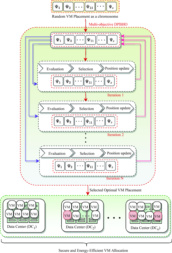
The VMs are allocated by utilizing Multi-objective DPBHO (i.e., M-DPBHO) which is an integration of proposed DPBHO algorithm and pareto-optimal selection procedure of Non-dominated Sorting based Genetic Algorithm (NSGA-II)²⁸. M-DPBHO comprises of steps: (i) initialization, (ii) evaluation, (iii) selection, and (iv) position update. As illustrated in Fig. 9, X VM allocations represented as stars/solutions: {$\Psi ^g_1$, $\Psi ^g_2$, …, $\Psi ^g_X$}$\in \Psi$ are randomly initialized, where g is the number of generation. These stars are evaluated using a fitness function $\eta (\Psi ^g)=$ [$f(\Psi ^g)_{\Xi _{{CDC}}}$, $f(\Psi ^g)_{PW_{{CDC}}}$, $f(\Psi ^g)_{PUE_{{CDC}}}$, $f(\Psi ^g)_{CFR_{{CDC}}}$, $f(\Psi ^g)_{RU_{{CDC}}}$] associated with security [Eq. (18)], power consumption [Eq. (25)], power usage effectiveness [Eq. (27)], carbon-foot rate [Eq. (28)], and resource utilization [Eq. (23)], respectively.

The population of stars is distributed into K sub-populations and local best blackholes ($\Psi ^k_{Lbest}$) are selected by estimating the fitness value using pareto-optimal selection procedure of NSGA-II. Thereafter, a second phase population is generated with the help of heuristic crossover [using Eq. (2)]. Similar to the local phase, a global best solution ($\Psi ^k_{Gbest}$) is observed from the second phase population using pareto-optimal procedure.

Therefore, to select the best VMP solution, a pareto-front selection procedure of NSGA-II is invoked that concedes all the objectives non-dominantly. A solution ($\Psi _i$) dominates other solution ($\Psi _j$), if its fitness value is better than that of $\Psi _j$ on atleast one objective and same or better on other objectives. The position update step of DPBHO [including Eq. (4)] along with Eqs. (5) and (6) for computing event horizon radius of local and global blackholes, respectively while Eqs. (7) and (8) are used to determine distance of a candidate solution from a local and global blackhole, respectively) is invoked to regenerate or update the existing population. Let a user job request ($\lambda$) is distributed into sub-units or tasks such as {$\tau _1$, $\tau _2$, …, $\tau _z$}$\in \lambda$. Eq. (29) is employed to select an appropriate VM for user application execution,

$$\begin{aligned} VM^{type}_{selected} = {\left\{ \begin{array}{ll} V_{S}, &{} {(\tau ^{\mathbb {R}}_{i} \le V_{S}^{\mathbb {R}} )} \\ V_{M}, &{} {( V_{S}^{\mathbb {R}}< \tau ^\mathbb {R}_{i} \le V_{M}^{\mathbb {R}})} \\ V_{L}, &{} {(V_{M}^{\mathbb {R}} < \tau ^\mathbb {R}_{i} \le V_{L}^{\mathbb {R}})} \\ V_{XL}, &{} \text {otherwise} \end{array}\right. } \end{aligned}$$

(29)

where $V_{S}^{\mathbb {R}}$, $V_{M}^{\mathbb {R}}$, $V_{L}^{\mathbb {R}}$ and $V_{XL}^{\mathbb {R}}$ represents small, medium, large and extra-large types of VM respectively, having capacity of resources $\mathbb {R} \in \{CPU, memory\}$ depending on their particular type, and $\tau ^\mathbb {R}_{i}$ represents resource utilization of $i$th task. If the maximum resource requirement of a task from $i$th task is lesser or equals to the resource capacity of $V_{S}$, then small type of VM is assigned to the task.

SaS-LM: operational design and complexity

Algorithm 2 elucidates a concise operational design of SaS-LM. Step 1 initializes list of VMs ($List_{\mathbb {V}}$), list of servers ($List_{\mathbb {S}}$), list of users ($List_{\mathbb {U}}$), and iteration counter (g) with O(1) complexity. Step 2 optimizes MFNN based predictor for resource usage analysis by invoking Algorithm 1 having O(XKt) complexity for t time-intervals. The steps 3–31 repeat for $\Delta t$, wherein any resource contention is detected and mitigated with the help of steps 4–9 with O(P) complexity. Step 10 receives live requests of users has O(1) complexity. Steps 11–13 select suitable VMs for requests execution with O(Q) complexity. X VM allocations are randomly initialized in step 14 with O(X) complexity.

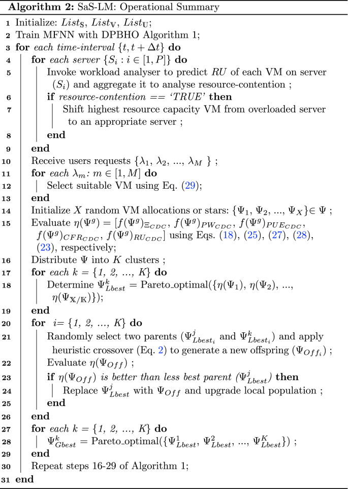
The cost values associated to five objectives is computed in step 15, where complexity is O(X) and step 16 distributes X VM allocations into K with O(1) complexity. The best VM allocation candidate is selected in steps 17–19 by invoking Pareto-optimal function have $O(X^2)$ complexity. The local population of VM allocations is upgraded using heuristic crossover in steps 20-26, consume O(K) complexity. Further, the cost values of second phase population (as mentioned in DPBHO Algorithm) is evaluated and global best candidate is selected in steps 27–29 with $O(K^2)$ complexity. Step 30 invokes set of instructions 16–29 of Algorithm 1, have O(KX) complexity. The total complexity of SaS-LM becomes $O(X^2K^2PQt)$.

Implementation

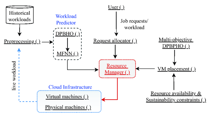
Figure 10 portrays a design and operational flow of the proposed model. Specifically, SaS-LM model is configured with the cooperative interaction of the distinguished modules discussed as follows:

Preprocessing (): The relevant numerical values of historical and live workloads are extracted and normalized to prepare input values for training of workload predictor.
Workload Predictor: This module is employed to estimate future resource usage on different servers with the help of multi-resource feed-forward neural network MFNN () module. This neural network is trained (offline) periodically to precisely estimate the approaching job requests in real-time to provide prior information to the Resource Manager () about the required amount of resources and alleviate any delay in job processing.
DPBHO (): This module implements Algorithm 1 for optimization of MFNN based predictor during training or learning process.
User (): User assigns job requests to Requests allocator () module at regular intervals for execution on different VMs. It also specifies deadline, cost, security, and resource availability constraints in Service Level Agreement (SLA).
Virtual machines (): As per the demand of the users, varying types of VM instances with specific configuration such as CPU, storage, bandwidth, operational status etc. are configured and allocated to servers.
Physical machines (): The varying types of servers configuration is defined by specifying their CPU, storage, bandwidth, operational status etc.
Resource availability and Sustainability constraints (): The security and sustainability constraints depict the computational models mentioned in Section “Secure and sustainable VM placement” which are considered non-dominantly to decide the most admissible allocation of VMs.
Multi-objective DPBHO (): This module appoints the VM placement strategy mentioned in Section “VM Management” to explore and exploit the population of random VM allocations and select the best VM placement.
Resource Manager (): This module receives essential information from different modules including Resource allocator (), Multi-objective DPBHO based VM placement, predicted resource capacity from MFNN (). Accordingly, it decides the allocation of available physical machines and manage the resources adaptively.