Hierarchical cloud architecture for identifying the bite of “Egyptian cobra” based on deep learning and quantum particle swarm optimization

Whereas snakes species identifications is the first process to treat a snake bite victim. Deep learning techniques have been used in many healthcare tasks, and achieve great success. This model uses deep learning techniques to identify the Egyptian cobra bite in an accurate manner based on an image of the marks of the bites. We build a dataset consisting of 500 images of cobra bites marks and 600 images of marks of other species of snakes that exist in Egypt. We utilize techniques such as transfer learning and data augmentation to boost the generalization and accuracy of our model.

Dataset collecting

We have faced a big challenge in that we have not found an available dataset that is convenient to our target. Also, the pictures of bite marks, that we need to train our model, are not generally available in a significant manner online because they must be shared after the agreement of the patient. So, we have to search online deeply to find pictures of bite marks of Egyptian cobra’s victims (this increases the difficulty of our mission). After searching in the zoology and medical scientific papers and online medical websites^19,23,24,25, we found 847 pictures of bite marks of the Egyptian cobra and 1005 images of other snakes bites marks, as shown in Fig. 2. This is not a very bad number considering the above difficulties, but we have to handle this challenge to get the best possible accuracy. We use data augmentation and transfer learning to handle this challenge. Whereas the size of the generated images in the data set is not the same and the sizes of images are different. So, we have changed the size of all the bite marks images into the same size of 1000 × 1000 pixels. For this, RGB reordering has been achieved and the input to the proposed model is presented as 1000 × 1000 × 3 image. The victims in this dataset are from different nationalities and ages, 73% of them are male and 27% are female, 54% of them are young and 46%of them are old people, part of them suffer from chronic diseases.

Bite marks of Egyptian cobra with two victims¹⁹.

Dataset pre-processing

Dataset enhancement

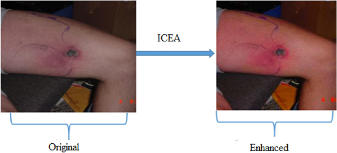
Compared with other image data in many research fields, most of the images of bitten persons by snakes are taken in poor countries, such as Egypt, Africa and India. So, the quality of these images is poor and the images backgrounds are usually complex. Image preprocessing is a very important process to remove damaged images, get rid of the effect of noise. During the process of generating the enhanced data set, contrast enhancement was applied on each image existed in the original dataset, using the image contrast enhancement algorithm (ICEA), as shown in Fig. 3. By this way, the noise in the original data set was eliminated and the best contrast was obtained. The ICEA is considered as one of the best image processing techniques used as a solution for the contrast enhancement issue. We used a new and efficient algorithm, for generating the enhanced dataset, which was proposed by Ying et al.²².

where R represents the result of enhancement, c represents the index of the three-color channels, and N is the number of images, W_i is the i-th image’s weight map, and P_i is the i-th image in the exposure set. Also, g is the Brightness Transform Function, and k_i is the exposure ratio.

Enhancement process for the dataset samples.

Dataset augmentation

Enhancing the generalization feature of the deep learning models is one of the most important challenges. Generalizability points to the performance of a model when dealing with data that it has not seen before (testing data) after training on previously seen data (training data). This needs a very large dataset to learn many features. However, there is sometimes a limited dataset. So, we have to handle this challenge to enhance the accuracy of the model. So, we the use data augmentation technique (DA). DA is a mechanism that can be utilized to artificially increase the size of a training data by generating modified data from the existing one. DA is proven that it achieves the best accuracy compared to other techniques that handle the limited dataset challenge. In this paper, flipping the image and zooming-in (zooming the image randomly by a certain degree) augmentation techniques are used to increase the dataset size, as shown in Table 3.

Transfer learning

Transfer learning is an efficient method in which we reuse a pre-trained deep learning model as a starting point to a model of a new task. In other word, a model trained previously on a task is reused on a second, related task to perform rapid progress while modeling the second task. By implementing the transfer learning on a new task, the model can achieve higher performance than training the model with a small amount of data. In this model, 3 popular pre-trained models were used to classify bite marks of the Egyptian Cobra from other species of snakes in Egypt: (1) VGG19, (2) VGG-16, (3) ResNet-101. VGG-19 consists of 19 layers, including 5 convolutional blocks and 3 fully-connected layers. Compared to VGG-16 model, VGG-19 is a deeper CNN architecture. ResNet-101 is a version of “Resnet” CNN. It is 101 layers depth with 33 residual blocks.

In our model, the convolution layer has a big importance because it does the feature extraction task. This layer utilizes the convolution operation which is alternative for the general matrix multiplication and is the basic building block of CNN. Also, the parameters of the convolution layer consist of a set of learnable filters, also called kernels. The basic task of the convolutional layer is to recognize the features in the regions of the input image and to generate a feature map.

This process depends on the technique of wandering a specific filter on the input image. The size of the filter can be 3 × 3, 5 × 5 or 7 × 7 pixels. The input to the next layer is created with the filter performed to the image. Activation maps happens as a result from this convolution process. Activation maps have local distinctive features.

Here, each convolution layer has a filter (m₁). The output of Layer l contains \({m}_{1}^{(l)}\) feature maps in \({Y}_{i}^{(l)}\), \({m}_{2}^{l}* {m}_{3}^{l}\) dimension. The i. feature map shown with \({Y}_{i}^{l}\) is calculated according to Eq. (1), \({B}_{i}^{(l)}\) is the deviation matrix, and \({K}_{i,j}^{l}\) is the filter dimension.

Pooling layers reduce the image dimension gradually so the number of the parameters and calculation complexity of the model are reduced. The pooling layer has two parameters, (l) the dimension of \({F}^{(l)}\) filter and \({S}^{(l)}\) step. The input of this layer is the data in the dimension \({m}_{1}^{l-1}* {m}_{2}^{l-1}* {m}_{3}^{l-1}\), provides \({m}_{1}^{l}* {m}_{2}^{l}* {m}_{3}^{l}\) output volume. The operation of the pooling layer is described in Eqs. (2), (3) and (4).

In the pooling operation, a v vector is decreased to a single scaler f (v) with pooling process f. There are two pooling types: average pooling, and max pooling. Max pooling is utilized here. FC layers turn the feature maps output of (1) final convolution or pooling layer into a unidimensional vector, (2) bind to one or more dense layers (3) update the weights, (4) and give the predicted of the final classification.

Proposed cloud architecture

We make use of cloud and edge computing techniques to boost the availability of our system and to decide at a very low time using edge computing technique. Whereas basic cloud unit is responsible for the training process for the model, whereas the storage and the computing capabilities of the cloud unit is convenient to perform this task in an efficient manner.

Edge computing structure

Edge computing is a technology utilized to enhance the efficiency of cloud computing architecture. In edge computing, specific parts of the system or services are transferred from the cloud unit to another close logical endpoint (the “edge”). The responsibility of the edge unit is to present fast services to the remote areas being served. When an application is started on the edge, it can provide a faster response to meet the requirements of real-time identification of Egyptian Cobra bite in remote areas, whereas Egyptian Cobra is able to kill a man in only 15 min. This requires fast identification of the bite. We suggest that in each state in Egypt, there is a number of edge computing units that contain the classifier application. This reduces the required time for the classification process because the classifier is closer to the user than to the cloud unit.

Novel re-training task in the cloud architecture

We have achieved 90.9% of accuracy, which is considered as an efficient result, not 100%, so it is normal for the system to perform sometimes wrong classifications. So, we suggest to re-train our model with the wrong predictions, whereas the edge computing units, where the classifier task is positioned, resend the wrong predictions to the cloud model, where the training process occurs, to retrain the model. This enhances the accuracy to the best level after a small period and increases the dataset size.

Determining the optimal number of edge nodes using quantum PSO algorithm

In each state, a number of edge nodes are deployed to present the classifier service to the users in this state. The optimal number of deployed edge nodes has to be determined based on some factors:

1. 1.

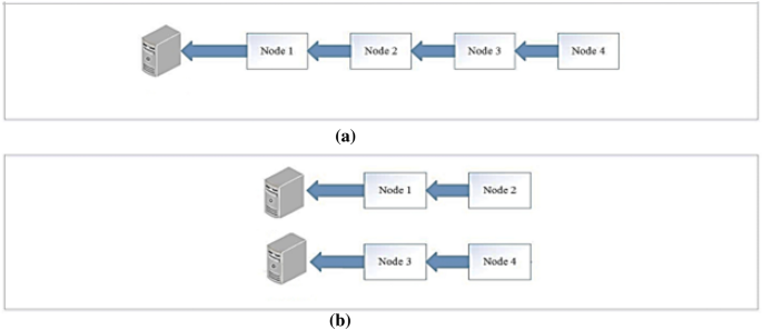
   Delay reduction: the Egyptian Cobra is able to kill a man in only 15 min, so the classification should be determined as quick as possible. The number of edge nodes affects the delay, as shown in Fig. 4, where in scenario a, if node 4 wants to send a data packet, it will wait for 4 hops delay. However, in scenario b, node 4 waits only 2 hops to reach an edge node. So, we can say that delay magnitude depends on the number of edge nodes, as shown in Eq. (5).

   $$D \alpha \frac{1}{k};$$

   (5)

   where D is the delay magnitude and k is the number of edge nodes.

2. 2.

   The bigger number of snake bites in a state is not necessarily a requirement for the more edge nodes existence. However, we suggest that these snake bites may be from non-venomous snakes. So, we consider the ratio of the number of deaths besides the number of blind cases or danger cases to the number of all snake bites in a state, as shown in Eq. (6). So, this ratio has to be close to the ratio of the number of edge nodes in this state to the number of edge nodes in all states. This leads to that each state contains the number of edge nodes that is convenient to its danger ratio.

   $$\frac{k}{K} – \frac{p + d}{n} \cong 0;$$

   (6)

   where k is the candidate number of edge nodes, K is the number of all edge nodes, p number of blind cases or any dangerous cases resulted from snakes bites in this states, d is the number of death cases resulted from snakes and n is the number of all snakes bites in this state.

3. 3.

   Cost (C): we must consider the cost of buying these edge nodes in each state to achieve the least cost.

The effect of edge nodes’ number on delay.

So, we have a maximization objective function to find the optimal number of edge nodes that achieves the best profit, as shown in Eq. (7).

We use particle swarm optimization (PSO) and quantum particle swarm optimization to solve the above optimization problem. So, the output of this process is an integer number which represent the optimal number of edge nodes to an area considering cost, delay and real danger range in this area.

Particle swarm optimization

PSO is an optimization algorithm inspired from birds flock when searching for the food. In PSO, the candidate solution is called a particle. Each particle has two variables: position and velocity, using them the particle moves through the search space towards the optimal solution¹⁶. PSO is an iterative technique. In each iteration, it checks the particle position (value) using the fitness function, and saves the particle’s local optimal value and the global optimal value for all particles. Based on the local and global optimal values, the particle updates the velocity that is utilized to calculate a new location for the particle (new candidate solution). The location and velocity of the particle are calculated using Eqs. (8) and (9), respectively. PSO has basic advantages : efficient solutions, ease of implementations, and computational and memory efficiency use.

where \({v}_{i}(t)\) is the velocity of particle \(i\) at round \(t\), \({x}_{i}(t)\) is the position of particle \(i\) at round \(t\), w is the inertia factor, \({c}_{1}\) and \({c}_{2}\) are two positive constants, \({P}_{i}\) is the local best of particle i, \(Pg\) is the global best of all particles, \({\varphi }_{1}\) and \({\varphi }_{2}\) are two random number between [0, 1].

Quantum PSO (QPSO)

The basic disadvantage of the traditional PSO algorithm is that it does not guarantee to reach the global optimal solution (Bergh 2001). Because of the small velocity of the particle, the particle is not able to cover the search space in an efficient manner. QPSO was proposed to handle this disadvantage of PSO. In quantum physics, the position and velocity of a particle could not be calculated at the same time. Therefore, the motion of a particle is described by a wave function denoted as ψ (x) that points to the probability of a particle to exist in a specific location (x) at a specific time. Based on Monte Carlo methodology, the motion state of a particle is described according to Eq. (10).

where PP_i is the local attractor of particle \(i\) that can be calculated based on Eq. (11), m_best is the mean personal best of all particles which can be determined according to Eq. (12), \(\alpha\) (Contraction–Expansion coefficient) can be tuned to determine the convergence speed,, u and b are random numbers between [0, 1] and \({P}_{i}\) is the local best of particle i.

where \({Pg}\) is the global best solution, φ is a random number between [0, 1],s is the swarm size and D is the number of dimensions in each particle. Compared to the traditional PSO, QPSO enhances greatly the global search ability and searches in wide space because of the exponential distribution of particle position, as shown in Eq. (10).