How do substitutability and effort asymmetry change resource management in coupled natural-human systems?

We formulate a mathematical model of RUs, public infrastructure provider (PIP), natural resources and PIs to find out how substitutability and effort asymmetry affect the general response, governance/management, and sustainability of CNHS. The model is built on the model developed in Muneepeerakul and Anderies (2017), with the key difference being the inclusion of a second resource (R2) and R2-specific PI (PI2) as Fig. 1b. A summary of key parameters and variables are provided in Table 1.
Adding substitutability and asymmetry to a CNHS model
Under the setting of two resources and two resource-specific PIs (see Fig. 1b), RUs decide how to distribute their effort to each resource due to their limited time and energy. The two resource-specific PIs are assumed to be governed by a single PIP, i.e., mimicking centralized governance structure. Consequently, the interactions between the two resource-PI subsystems are indirectly linked by the behavior of RUs and the policy of PIP (to be distinct from cases in which the two resources interact directly as in predator-prey situations). Specifically, the effects of substitutability and asymmetry are captured in a utility calculation, which makes use of CES (constant elasticity of substitution) production function. CES production function has traditionally been used for analyzing conditions of natural or human capitals in economics, and its generic form is as follows:
$$U = A\left[ {\alpha X_1^\beta + \left( {1 – \alpha } \right)X_2^\beta } \right]^{\frac{1}{\beta }},$$
where α (0 ≤ α ≤ 1) and β (β ≤ 1) (these are the ranges of values that make sense economically (Kemfert, 1998; Markandya and Pedroso-Galinato, 2007) capture the effects of asymmetry and substitutability, respectively. α reflects how much RUs distribute their effort shares on one resource (in this case, Resource 1 with a payoff X1) to derive their wellbeing. When α equals 0.5, the effort shares are symmetric: RUs distribute the same amount of time or energy on two resources. Asymmetry occurs when α increases or decreases from 0.5. When α is one or zero, RUs only work with Resource 1 or 2, i.e., the single-resource setting is resumed. Our model does not simulate these conditions because substitutability and asymmetry are irrelevant when only one resource exists. β describes how substitutable two resources are. β is 1 if two resources are perfectly substitutable, and substitutability between the two reduces with smaller or negative β values.
An intriguing aspect is that RUs can observe the asymmetry in efforts of other RUs and adjust their own, through such mechanisms as replicator dynamics or optimization. To keep the dimensionality of the model low and its result interpretation clear, α is currently treated as a parameter in the present analysis, but such dynamical aspects of α call for additional future analyses.
Natural resource dynamics
There are two resources (R1 and R2) in this model, whose dynamics are captured by the following equations:
$$\frac{{dR_i}}{{dt}} = G_i\left( {R_i} \right) – A_i\left( {R_i,I_i,U,\alpha _i} \right)\;\;\;\;\;\;\;\;{\mathrm{for}}\;i = \left\{ {1,\,2} \right\},$$
where Gi(Ri) is the natural process of resources, and Ai(Ri, Ii, U, αi) is the harvest of natural resources by RUs. Gi(Ri) is assumed to take a simple form of g −lRi, where g is the natural growth rate of resources and l is the natural death rate of resources. To highlight the interactions between different entities and facilitate result interpretation, we set g and l of the two natural resources to be identical. This configuration prevents individual characteristics of natural resources to become a main driver of the results. The amount of RUs’ Resource i harvest is proportional to the number of RUs (N), a fraction of time RUs participate inside the system (U), levels of natural resources (Ri), productivity of PI per person (Hi(Ii)), and how much RUs share their effort to different resources (αi; α1 = α, α2 = 1−α). Putting them all together, we obtain that Ai(Ri, I, U, αi) equals αiUNRiHi(Ii).
Public infrastructure dynamics
In this model, public infrastructure PI1 and PI2 are specific to Resources 1 and 2, respectively. Each PI is not directly involved in the other resource, and its state (represented by variables I1 and I2) individually changes over time. PIs naturally age over time and require continuous maintenance by the participation of RUs. Then,
$$\frac{{dI_i}}{{dt}} = M_i\left( {R_i,I_i,U,\alpha _i} \right) – \delta I_i\;\;\;\;\;\;\;\;{\mathrm{for}}\;i = \left\{ {1,\,2} \right\},$$
where Mi(Ri, Ii, U, αi) is the maintenance of each PI by the PIP, and δ is a natural decay rate of PIs. PIs are sustained well when the PIPs invest a large enough portion from tax, and RUs sufficiently harvest natural resources. Mi(Ri, Ii, U, αi) will be explained in the social dynamics section below. All the parameters of PI1 and PI2 are the same, again, to highlight the interactions between different entities and facilitate result interpretation. Note that PIs are not directly coupled to each other; they are indirectly coupled through decision-making processes of the PIP and RUs. I1 and I2 are then mapped into a productivity-related term through the productivity function Hi(Ii):
$${H_i}({I_i}) = \left\{ {\begin{array}{*{20}{c}}{0,}&\quad{{I_i}\,<\,{I_0}}\\{h\frac{{{I_i} – {I_0}}}{{{I_m} – {I_0}}},}&{{I_0} \le {I_i}\,<\,{I_m}\quad{\mathrm{for}}\,i =\{ 1,2\} ,}\\{h,}&\quad{{I_i} \ge {I_m}}\end{array}} \right.$$
where h is a maximum harvest productivity per person. Most PIs do not function when their states are less than a certain threshold (I0). Moreover, there is usually the limit to the productivity of PI, which is assumed to remain the same after the state reaches a threshold (Im).
Social dynamics and decision-making
To capture the social evolution, we make use of several established equations and relationships from social science to mathematically define social responses and decision-making dynamics. For RUs, replicator equations–from evolutionary game theory (Muneepeerakul and Anderies, 2017)–and CES production function are combined to model changes in the RUs’ behaviors.
A generic form of the replicator equation for a frequency of strategy i (xi) is \(\dot x_i = x_i\left( {\pi _i – \phi } \right)\), where πi is a payoff a user earns from strategy i, and ϕ is an averaged payoff. In this model, RUs have two options: to stay inside the system by participating in crop farming (U) with a payoff πU and to work outside the system (W; U+W = 1) with a wage w (=πW). When working inside the system, a RU must pay a fraction C of farming revenue to the PIP (Link 3 in Fig. 1). Then, the replicator equation for our model is as follows:
$$\frac{{dU}}{{dt}} = rU\left( {1 – U} \right)\left( {\pi _U – w} \right)$$
When multiple natural resources have substitutable relations, the calculation of πU is not simply the sum of each natural resource revenue. It is here where we incorporate the concept of substitutability from economics through CES production function.
In this paper, we focus on the effects of α and β in the production function, which represent degrees of effort asymmetry and substitutability, respectively. Specifically, we write πU as follows:
$$\pi _U = \left( {1 – C} \right)\left[ {\alpha \left( {p_1R_1H_1\left( {I_1} \right)} \right)^\beta \,+ \,\left( {1 – \alpha } \right)\left( {p_2R_2H_2\left( {I_2} \right)} \right)^\beta } \right]^{\frac{1}{\beta }},$$
where piRiHi(Ii) is a payoff which RUs earn from resource i.
Maintenance of infrastructure i (Mi(Ri,Ii,U,αi)) is assumed to depend on various factors described in preceding paragraphs. First, it depends on how much income RUs extract from resource i, namely αipUNRiHi(Ii). RUs then contribute a fraction C (which is decided on by the PIP) of this income to the PIP. The PIP decides on what fraction yi of these RU contributions will be invested in the maintenance of infrastructure i. Finally, the maintenance function of PIi is Mi(Ri, Ii, U, αi) = μyiCαipUNRiHi(Ii), where μ is an efficiency parameter of PIP investment. The payoff of PIP is πPIP = CpUN[(1 − y1)αR1H1(l1) + (1 − y2)(1 − α)R2H2(I2)].
Coupled dynamics
To address our research questions, we conduct numerical simulations (trapezoidal numerical approximation) of the above dynamical model with combinations of policy parameters (y1, y2 and C) for a wide range of substitutability (β) and asymmetry (α) settings. We then analyze the results for cases in which the coupled system is sustained in the long run or collapses at different degrees of shocks to Resource 1. To clearly see the interplay between disturbance, effort asymmetry, substitutability, system performance, and sustainability, we run the simulations long enough, until the system is stabilized. Then, we subject the system to a shock in the form of a drop in the availability of Resource 1. By applying shocks only to Resource 1, our analysis highlights the roles played by the substitutability and asymmetry of natural resources.
Defining sustainability and viable policy for CNHS
In what follows, CNHS is said to be “sustained in the long run” if the following conditions are met: 1) Some RUs remain in the system and participate in resource-related labors (U* > 0), and 2) Investing in the maintenance of PIs to sustainably manage natural resources is more profitable for PIP than the alternative option (πP ≥ wP), ensuring sufficient incentives for the PIP to participate in the system. In other words, these definitions state that both types of social agents (RUs and PIP) must be sufficiently satisfied for the system to be “sustained in the long run”.
For given α and β values, a large number of y1, y2 and C combinations (132,651 in total)—the combination {y1, y2, C} a policy (see Table 1)—are prescribed to the system. The policies that satisfy the two sustainability conditions above—which we dub “viable policies”—constitute a “cloud” in the y1−y2−C policy space (see Fig 2a–c). In certain parts, both I1 and I2 are functioning, but in others, only one of either I1 or I2 functions. Only I1 functions in all cloud points when α is close to one, only I2 functions in all cloud points when α is close to zero (see Fig. 2a), and both I1 and I2 function in all cloud points when α is 0.5 (see Fig. 2c). As α moves from 0.5 (symmetric condition) to either of its extremes close to 0 or 1 (asymmetric conditions), the viable-policy cloud bifurcates into two clusters, one of which includes policies corresponding to only one functioning PI.
a a viable policy cloud in y1–y2–C policy space at α = 0.1 (extremely asymmetric condition), β = 1 (highly substitutable condition) and no disturbance case. b a viable policy cloud in y1–y2–C policy space at α = 0.3 (moderately asymmetric condition), β = 1 and no disturbance case. c a viable policy cloud in y1–y2–C policy space at α = 0.5 (symmetric multiple-resource condition), β = 1 and no disturbance case. d 3D bar graph which sums up the points in policy clouds on behalf of policy flexibility for every α and β combination. Each red box represents the number of points inside the clouds in (a–c). Color bars for (a), (b) and (c) are payoffs of PIP in each y1–y2–C policy design. The blue dots are projections of the clouds to y1–y2, y1–C and y2–C planes
Sustainability of CNHS is also relevant to uncertain disturbances. The world does not simply stay in the equilibriums but is often perturbed by various external forces: natural (e.g., floods, droughts, earthquakes, etc.) or social forces (e.g., price changes, migration, policy changes, etc.) (Anderies et al., 2004). In this research, we drop a state of one resource (Resource 1) to certain levels to directly evaluate sustainability when one resource is in short. A policy design which seemed to be “viable” may fail when disturbed. We analyze whether CNHS is still well-sustained after experiencing disturbances, making a comparison to cases without any shock.


