Multi-objective optimization of water resources allocation in Han River basin (China) integrating efficiency, equity and sustainability
Conceptual framework
In this study, we propose a comprehensive water resources management model to define how water can be optimally allocated to achieve the best comprehensive benefit. The proposed model consists of 3 main parts: (1) available water resources and water demand projection; (2) multi-objective optimization of water resources allocation; (3) analysis and evaluation of allocation schemes.
According to hydrological patterns, geographical positions and the requirements of production management departments, 15 water-intakes are segmented in the study. Besides, the water connections, water acquisition and water-break are determined through investigations and official data. Based on the runoff depth, collection area, reservoir operation and inter-basin water transfer projects, the available water resources in each water-intake can be attained. Correspondingly, the water demand of each sector in the planning level year in each water-intake can be predicted.
Furthermore, the optimization objectives are defined in terms of regional sustainable development. The model is supposed to promote high-quality water utilization in objective conditions while tackling the issues of the uneven temporal and spatial water resources distribution, the incoordination between the development of economy and society and the distribution of water resources. Water allocation problems involve complex political, economic, social and environmental elements. Single-targeted water resources distribution does not meet the demand of advanced development of society and economy. Therefore, a water management model needs to address a multi-objective problem.
Taking the above-mentioned development issues into consideration, the general objective of the research is to establish an integrated water allocation scheme for attaining efficiency, equity and ecological sustainability. Under the sustainability constraint, the objectives are maximizing economic interest and water allocation equity. The conceptual framework (Fig. 4) of the proposed methodology, utilized here to identify the optimal quantity of water in the network, demonstrates a practicable mechanism for the appropriate allocation of water resources.
Optimal water resources allocation model
The ensuing assumptions were declared without conflicts for the water allocation condition in the river basin system before starting the model.
-
(1)
The river basin administrative agency takes charge of the water allocation and management, and the water allocated to each water-intake is perceived as tenable and well-grounded.
-
(2)
The managers have a profound comprehension as to how the model works, e.g. the objective functions and the constraints, and each water-intake water manager conducts in accordance with the leader.
-
(3)
Ecological water is essential for fish, wildlife, water recreation and other related environmental resources. The ecological water demand is necessary to guarantee during the allocation process however economic activities perform6. In this study, the minimum ecological water demand is considered for water resources allocation, and the instream flows (ecology sustainability) are guaranteed first and then the remaining water is allocated into different water use sectors and regions, which is a conventional approach in practice28. Since the water consumption coefficient of each water use sector is different, and the economic activities are dependent on water availability, the overall water return will be different after economic production activities, and the water consumption of each water use sector in the upstream area will have an impact on the water volume at the outlet section of the area28. To meet the sustainability in the process of river water intake, which is set as the constraint in the model, the total water supply to the next area will be affected accordingly. Therefore, from upstream to downstream, the water resources allocation process in the upstream area will affect the water resources allocation in the downstream area.
-
(4)
Water-rights trading does not exist in the water-intakes or sectors.
To clearly present the proposed model, the main notations are listed in Table 2.
Objective functions
Objective 1: Maximizing economic efficiency
Water resources are the vital element for human survival and economic construction. The development of social economy is closely tied to water resources management, which lays the foundation of the former. Humans need to create monetary output as much as possible to seek high-quality development. Consequently, the first objective function is to maximize economic efficiency. For a typical hydrological year with a determined hydrological situation, we neglect the subtle difference between economic efficiency and economic benefit which are coincided generally29. The calculation of economic benefit is very easy and has been widely used in complex water resources allocation process. In the real world, a water consumption sector might have feedbacks to other sectors. The specific forward and backward linkages are not clear and quantitative in the state-of-the-art studies. For the simplicity of predicting water demands and allocating water resources, we divide the sectors into domesticity, industry, agriculture and ecology, which has been a general method in water resources planning and management28,30. In this study, we selected the gross economic interest to represent the efficiency.
$$f_{1} (x) = \max \;\left( {\sum\limits_{t = 1}^{T} {\sum\limits_{i = 1}^{I} {\sum\limits_{j = 1}^{J} {(NER_{i,j} \cdot x_{i,j}^{t} )} } } } \right)$$
(1)
where \(NER_{i,j}\) refers to the net economic return per unit of water quantity of jth sector in ith water-intake; \(x_{i,j}^{t}\) refers to the water allocated to the jth sector in ith water-intake in tth time. \(T\) refers to the total number of months during calculation, I refers to the total number of water-intakes, and J refers to the total number of water use sectors.
Objective 2: Maximizing the water allocation equity
Equity means equal access to water and the benefits of water use. The relative fairness of water use between regions is the basic principle in water resources allocation, and also the core issue of sustainable use of water resources and coordinated development at the regional level. The river authority needs to consider equity in the water allocation process to ensure the balanced development in each water-intake.
Gini coefficient, proposed by Italian economist Gini31, has been generally utilized to evaluate the inequality degree in income distribution. In addition to the evaluation of equality in the distribution of wealth in the economic society, it can be applied to various aspects of the assessment of the fairness of distribution in other disciplines, e.g. balance between water and soil32.
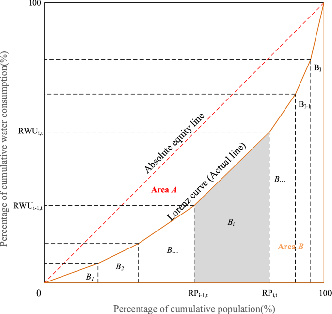
The Lorenz curve for water resources allocation is presented in Fig. 5, where X axis refers to cumulative population share, and Y axis denotes cumulative water consumption, A represents the area between the absolute equity line and Lorenz curve, and B denotes the area below the Lorenz curve. Then the Gini coefficient is equal to A/(A + B)33.
In water resources allocation, Y axis denotes cumulative water consumption, X axis refers to cumulative population share, cumulative gross domestic product share and cumulative available water resources share, respectively. In this study, we use trapezoidal area method to calculate the areas of A and B. According to the water allocation scheme, we can plot the Lorenz curve for water resources allocation. The value of Gini coefficient is equal to A/(A + B). As A + B = 1/2, the Gini coefficient is also equal to 1 − 2B3.
We choose three types of Gini coefficients to evaluate the equality of water resources allocation, i.e., (1) Gini coefficient between population and water consumption (PGC), representing the diversity of per capita water consumption among different regions; (2) Gini coefficient between gross domestic product (GDP) and water consumption (GGC), reflecting the difference between per unit of GDP in different regions; (3) Gini coefficient between available water resources and water consumption, (WGC), denoting water uses’ degree of dependence on other regions. These three kinds of Gini coefficients are calculated as below:
(1) EPGC
$$EPGC = \sum\limits_{t = 1}^{T} {\frac{{PGC_{t} }}{T}}$$
(2)
$$PGC_{t} = 1 – \sum\limits_{i = 1}^{I} {(RWU_{i,t} + RWU_{i – 1,t} ) \cdot (RP_{i,t} + RP_{i – 1,t} )}$$
(3)
$$EPGC = \sum\limits_{t = 1}^{T} {\frac{{PGC_{t} }}{T}} = 1 – \sum\limits_{t = 1}^{T} {\sum\limits_{i = 1}^{I} {\frac{{(RWU_{i,t} + RWU_{i – 1,t} ) \cdot (RP_{i,t} + RP_{i – 1,t} )}}{T}} }$$
(4)
where \(EPGC\) denotes the average of \(PGC\), \(PGC_{t}\) denotes the \(PGC\) in tth time, \(T\) refers to the total number of months during calculation; I refers to the total number of water-intakes, \(RWU_{i,t} (RP_{i,t} )\) refers to the cumulative percentage of water consumption (population) in ith water-intake in tth time; \(RWU_{i,t}\) and \(RP_{i,t}\) are equivalent to zero in the initial stage.
(2) EGGC
$$EGGC = \sum\limits_{t = 1}^{T} {\frac{{GGC_{t} }}{T}} = 1 – \sum\limits_{t = 1}^{T} {\sum\limits_{i = 1}^{I} {\frac{{(RWU_{i,t} + RWU_{i – 1,t} ) \cdot (RG_{i,t} + RG_{i – 1,t} )}}{T}} }$$
(5)
where \(EGGC\) denotes the average of \(GGC\), \(GGC_{t}\) denotes the \(GGC\) in tth time, \(RG_{i,t}\) refers to the cumulative percentage of GDP in ith water-intake in tth time, \(RG_{i,t}\) is equivalent to zero in the initial stage.
(3) EWGC
$$EWGC = \sum\limits_{t = 1}^{T} {\frac{{WGC_{t} }}{T}} = 1 – \sum\limits_{t = 1}^{T} {\sum\limits_{i = 1}^{I} {\frac{{(RWU_{i,t} + RWU_{i – 1,t} ) \cdot (RW_{i,t} + RW_{i – 1,t} )}}{T}} }$$
(6)
where \(EWGC\) denotes the average of \(WGC\), \(WGC_{t}\) denotes the \(WGC\) in tth time, \(RW_{i,t}\) refers to the cumulative percentage of available water resources in ith water-intake in tth time, \(RW_{i,t}\) is equivalent to zero in the initial stage.
The second objective function is to minimize the comprehensive Gini coefficient to consider the impacts of various indexes on water consumption.
$$f_{2} (x) = \min \;(\omega_{1} \cdot EPGC + \omega_{2} \cdot EGGC + \omega_{3} \cdot EWGC)$$
(7)
where \(f_{1} (x)\) denotes the comprehensive Gini coefficient, \(\omega_{i} (i = 1,\;2,\;3)\) denotes the weighting coefficient and the sum of \(\omega_{i} (i = 1,\;2,\;3)\) is equivalent to one. The impacts of population, GDP, and available water resources on water consumption can be viewed as equally important34. Hence, \(\omega_{i} (i = 1,\;2,\;3)\) are equal to 1/3 in this paper.
Constraints
The main constraints are as follows.
(1) Water availability constraints
$$\sum {x_{i,j}^{t} } \le AW_{i}^{t}$$
(8)
where \(x_{i,j}^{t}\) refers to jth water use sector in ith water-intake in tth time, \(AW_{i}^{t}\) represents the available water in ith water-intake in tth time.
(2) Reservoir water balance constraints
For the reservoir, the change of storage capacity is captured by water balance:
$$V_{k}^{t + 1} = V_{k}^{t} + (I_{k}^{t} – O_{k}^{t} ) \times \Delta T(t) – L_{k}^{t}$$
(9)
where \(V_{k}^{t + 1}\) and \(V_{k}^{t}\) denote the storage capacity of kth reservoir in (t + 1)th and tth time, respectively; \(I_{k}^{t}\) and \(O_{k}^{t}\) refer to the reservoir inflow and discharge of kth reservoir in tth time, respectively. In this study, we also set the discharge of each reservoir as the decision variables, \(y_{i,j}^{t}\). \(\Delta T(t)\) refers to the time interval; and \(L_{k}^{t}\) denotes the water loss of kth reservoir in tth time.
(3) Reservoir storage capacity constraints
For the reservoir, its operation rule is subject to the physical property and comply with the requirements in practical management, thus the real-time storage capacity is constrained by the maximal and minimal storage capacity:
$$V_{k,\min }^{t} \le V_{k}^{t} \le V_{k,\max }^{t}$$
(10)
where \(V_{k,\min }^{t}\) refers to the lower bound of kth reservoir in tth time, usually the dead storage capacity; \(V_{k,\max }^{t}\) refers to the upper bound of kth reservoir in tth time, usually the maximum storage capacity below the normal storage water level in the non-flood season and below the flood-control water level in the flood season, respectively.
(4) Reservoir outflow discharge
$$y_{i,j}^{t} \le q_{\max i,j}^{t}$$
(11)
where \(y_{i,j}^{t}\) refers to the discharge of the jth reservoir in ith water-intake in tth time; \(q_{\max i,j}^{t}\) refers to the discharge capacity of the jth reservoir in ith water-intake in tth time.
(5) Water demand constraints
For water use sectors in each water-intake, the amount of the water supplied shouldn’t exceed its expectation:
$$x_{i,j}^{t} \le Wd_{i,j}^{t}$$
(12)
where \(Wd_{i,j}^{t}\) denotes the water demand of the jth water use sector in ith water-intake in tth time.
(6) Non-negative constraints
The water allocated to the jth water use sector in ith water-intake in tth time shouldn’t be less than zero:
$$\begin{array}{*{20}l} {x_{i,j}^{t} \ge 0} \hfill \\ {y_{i,j}^{t} \ge 0} \hfill \\ \end{array} .$$
(13)
Global model
In this study, the optimal water resources allocation model can be formulated as shown below:
$${\text{Objective}}\quad \quad \left\{ {\begin{array}{*{20}l} {f_{1} (x) = \max \;\left( {\sum\limits_{t = 1}^{T} {\sum\limits_{i = 1}^{I} {\sum\limits_{j = 1}^{J} {(NER_{i,j} \cdot x_{i,j}^{t} )} } } } \right)} \hfill \\ {f_{2} (x) = \min \;(\omega_{1} \cdot EPGC + \omega_{2} \cdot EGGC + \omega_{3} \cdot EWGC)} \hfill \\ \end{array} } \right.$$
(14)
$${\text{Subject}}\,{\text{to}}\quad \quad \left\{ {\begin{array}{*{20}l} {\sum {x_{i,j}^{t} } \le AW_{i}^{t} } \hfill \\ {V_{k}^{t + 1} = V_{k}^{t} + (I_{k}^{t} – O_{k}^{t} ) \times \Delta T(t) – L_{k}^{t} } \hfill \\ {V_{k,\min }^{t} \le V_{k}^{t} \le V_{k,\max }^{t} } \hfill \\ {y_{i,j}^{t} \le q_{\max i,j}^{t} } \hfill \\ {x_{i,j}^{t} \le Wd_{i,j}^{t} } \hfill \\ {x_{i,j}^{t} \ge 0} \hfill \\ {y_{i,j}^{t} \ge 0} \hfill \\ \end{array} } \right.$$
(15)
where \(f_{1} (x)\) and \(f_{2} (x)\) are the objective functions, \(x_{i,j}^{t}\) refer to the design variables and the remaining formulas are the constraints. More detailed information on the programming model can be found in “Objective functions” section and “Constraints” section.
Optimization algorithm
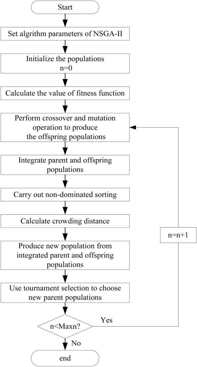
The well-known NSGA-II algorithm (Fast non-dominated sorting genetic algorithm), proposed by Deb et al.35, has been extensively applied in multi-objective optimization issues. The employed elitist strategy in this algorithm can preserve the diversity of strategies, so as to enhance the operation speed and improve the robustness36. It achieves fast convergence by utilizing the strategies of crowding distance and non-dominated sorting rank37. Meanwhile, it reduces the complexity of the traditional non-inferior ranking genetic algorithm and becomes the performance benchmark of other multi-objective optimization algorithms38. Due to the above advantages, the evolutionary approach to find the optimal solutions to complex multi-objective optimization problems has been widely used in water resources management16,34,37,38,39. Therefore, NSGA-II is used in this study to trade off efficiency and equity. The flowchart of NSGA-II algorithm is shown in Fig. 6, and the detailed procedure can be found in the reference35. The population size, the number of the maximal generation, the crossover probability and the mutation probability were set as 700, 600, 0.9 and 0.1, respectively. It was noticed that the parameters of the NSGA-II could be obtained using an intensive trial-and-error procedure for producing converged results40.
Decision-making method
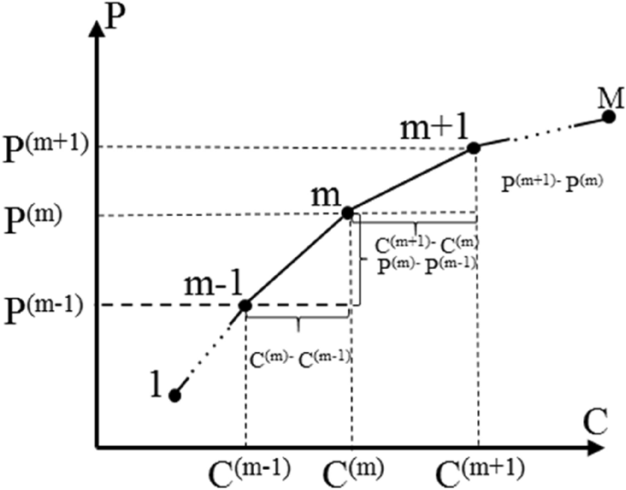
Generally, there is a trade-off relationship in the Pareto front. How to select a balance point between optimization objectives is an important issue. To achieve this, we usually need to find a solution that is acceptable to each objective with minimum deviation. The cost performance method proposed by Wang et al.41 is utilized to select the solution (Fig. 7).
Let \(M\) be the number of Pareto solution sets, which can be sequenced in order. \(P^{(m)}\) is the value of the first objective function of the mth Pareto solution, \(m \in \{ 1,2, \ldots M\}\); \(C^{(m)}\) is the value of the second objective function of the mth Pareto solution, \(m \in \{ 1,2, \ldots M\}\), then the average change rate of the above two objectives is:
$$k_{1}^{(m)} = \frac{1}{2}\left( {\frac{{P^{(m + 1)} – P^{(m)} }}{{C^{(m + 1)} – C^{(m)} }} + \frac{{P^{(m)} – P^{(m – 1)} }}{{C^{(m)} – C^{(m – 1)} }}} \right),m \in \{ 2,3, \ldots M – 1\}$$
(16)
$$k_{2}^{(m)} = \frac{1}{2}\left( {\frac{{C^{(m + 1)} – C^{(m)} }}{{P^{(m + 1)} – P^{(m)} }} + \frac{{C^{(m)} – C^{(m – 1)} }}{{P^{(m)} – P^{(m – 1)} }}} \right),m \in \{ 2,3, \ldots M – 1\}$$
(17)
where \(k_{1}^{(m)}\) and \(k_{2}^{(m)}\) refer to average change rate of the first objective and the second objective, respectively. Especially, when m is equal to 1 or M, the average change rate is:
$$k_{1}^{(1)} = \frac{{P^{(2)} – P^{(1)} }}{{C^{(2)} – C^{(1)} }}$$
(18)
$$k_{2}^{(1)} = \frac{{C^{(2)} – C^{(1)} }}{{P^{(2)} – P^{(1)} }}$$
(19)
$$k_{1}^{(M)} = \frac{{P^{(M)} – P^{(M – 1)} }}{{C^{(M)} – C^{(M – 1)} }}$$
(20)
$$k_{2}^{(M)} = \frac{{C^{(M)} – C^{(M – 1)} }}{{P^{(M)} – P^{(M – 1)} }}$$
(21)
Based on the above results, the sensitivity ratios are calculated by
$$\delta_{1}^{(m)} = \frac{{k_{1}^{(m)} }}{{P^{(m)} }},m \in \{ 1,2, \ldots ,M\}$$
(22)
$$\delta_{2}^{(m)} = \frac{{k_{2}^{(m)} }}{{C^{(m)} }},m \in \{ 1,2, \ldots ,M\}$$
(23)
where \(\delta_{1}^{(m)}\) and \(\delta_{2}^{(m)}\) refer to the sensitivity ratios of the first objective and the second objective, respectively. For the convenience of comparison, the above results need to be dimensionless, the specific expression is
$$\varepsilon_{1}^{(m)} = \frac{{\delta_{1}^{(m)} }}{{\sum\nolimits_{m = 1}^{M} {\delta_{1}^{(m)} } }},m \in \{ 1,2, \ldots ,M\}$$
(24)
$$\varepsilon_{2}^{(m)} = \frac{{\delta_{2}^{(m)} }}{{\sum\nolimits_{m = 1}^{M} {\delta_{2}^{(m)} } }},\;m \in \{ 1,2, \ldots ,M\}$$
(25)
where \(\varepsilon_{1}^{(m)}\) and \(\varepsilon_{2}^{(m)}\) refer to the dimensionless sensitivity ratios of the first objective and the second objective, respectively. The formulas for preference degrees based on sensitivity ratios are as follows:
$$\omega_{1}^{(m)} = \frac{{\varepsilon_{1}^{(m)} }}{{\varepsilon_{1}^{(m)} + \varepsilon_{2}^{(m)} }},\;m \in \{ 1,2, \ldots ,M\}$$
(26)
$$\omega_{2}^{(m)} = \frac{{\varepsilon_{2}^{(m)} }}{{\varepsilon_{1}^{(m)} + \varepsilon_{2}^{(m)} }},\;m \in \{ 1,2, \ldots ,M\}$$
(27)
where \(\omega_{1}^{(m)}\) and \(\omega_{2}^{(m)}\) refer to the preference degrees of mth Pareto solution for the first objective and the second objective, respectively.
