Plotting Golf Courses in R with Google Earth | by Adam Beaudet | May, 2024

Once we’ve finished mapping our hole or course, it is time to export all that hard work into a KML file. This can be done by clicking the three vertical dots on the left side of the screen where your project resides. This project works best with geoJSON data, which we can easily convert our KML file to in the next steps. Now we’re ready to head to R.
The packages we will need to prepare us for plotting are: sf (for working with geospatial data), tidyverse (for data cleaning and plotting), stringr (for string matching), and geojsonsf (for converting from KML to geoJSON). Our first step is reading in the KML file, which can be done with the st_read() function from sf.
# load libraries
library(sf)
library(tidyverse)
library(stringr)
library(geojsonsf)kml_df <- st_read("/Users/adambeaudet/Downloads/erin_hills.kml")
Great! Now we should have our golf course KML data in R. The data frame should have 2 columns: Name (project name, or course name in our case), and geometry (a list of all individual points comprising the polygons we traced). As briefly mentioned earlier, let’s convert our KML data to geoJSON and also extract the course name and hole numbers.
# convert from KML to geoJSON
geojson_df <- st_as_sf(kml_df, "POLYGON")# extracting course name and hole number from polygon name
# assuming "course_hole_element" naming convention is used for polygons
geojson_df$course_name <- str_match(geojson_df$Name, “^(.+)_hole”)[,2]
geojson_df$hole_num <- gsub(“.*_hole_(\\d+)_.*”, “\\1”, geojson_df$Name)
To get our maps to point due north we need to project them in a way that preserves direction. We can do this with the st_transform() function.
# define a CRS for so map always points due north
crs <- "+proj=lcc +lat_1=33 +lat_2=45 +lat_0=39 +lon_0=-96 +x_0=0 +y_0=0 +datum=WGS84 +units=m +no_defs"# transform data to CRS
geojson_df <- st_transform(geojson_df, crs)
We’re almost ready to plot, but first, we need to tell ggplot2 how each polygon should be colored. Below is the color palette my project is using, but feel free to customize as you wish.
Optional: in this step we can also calculate the centroids of our polygons with the st_centroid() function so we can overlay the hole number onto each green.
geojson_df <- geojson_df %>%
mutate(color = case_when(
grepl(“_tee$”, Name) ~ “#57B740”,
grepl(“_bunker$”, Name) ~ “#EDE6D3”,
grepl(“_water$”, Name) ~ “#2243b6”,
grepl(“_fairway$”, Name) ~ “#57B740”,
grepl(“_green$”, Name) ~ “#86D14A”,
grepl(“_hazard$”, Name) ~ “#094d1d”
)) %>%
mutate(centroid = st_centroid(geometry))
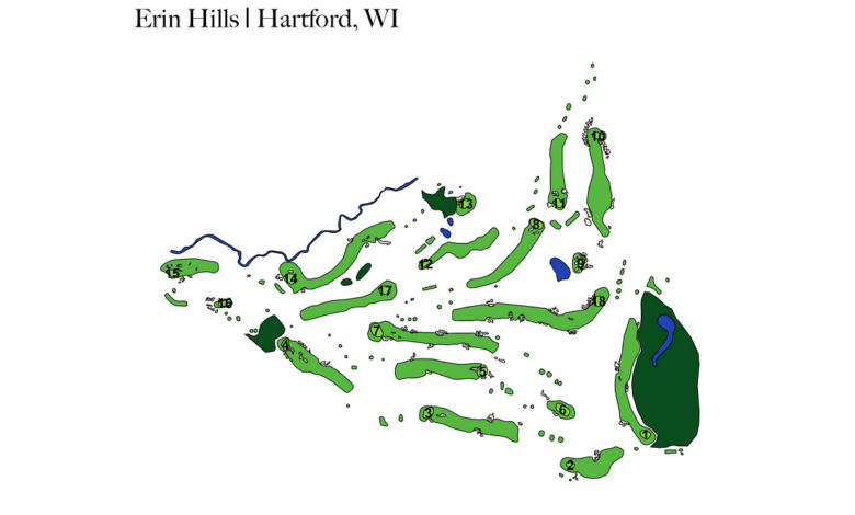
We’re officially ready to plot. We can use a combination of geom_sf(), geom_text(), and even geom_point() if we want to get fancy and plot shots on top of our map. I typically remove gridlines, axis labels, and the legend for a cleaner look.
ggplot() +
geom_sf(data = geojson_df, aes(fill = color), color = "black") +
geom_text(data = filter(geojson_df, grepl("_green", Name)),
aes(x = st_coordinates(centroid)[, 1],
y = st_coordinates(centroid)[, 2],
label = hole_num),
size = 3, color = "black", fontface = "bold", hjust = 0.5, vjust = 0.5) +
scale_fill_identity() +
theme_minimal() +
theme(axis.title.x = element_blank(),
axis.title.y = element_blank(),
axis.text.x = element_blank(),
axis.text.y = element_blank(),
plot.title = element_text(size = 16),
panel.grid.major = element_blank(),
panel.grid.minor = element_blank()) +
theme(legend.position = "none") +
labs(title = 'Erin Hills | Hartford, WI')
And there you have it — a golf course plotted in R, what a concept!
To view other courses I have plotted at the time of writing this article, you can visit my Shiny app: https://abodesy14.shinyapps.io/golfMapsR/
If you followed along, had fun in doing so, or are intrigued, feel free to try mapping your favorite courses and create a Pull Request for the golfMapsR repository that I maintain: https://github.com/abodesy14/golfMapsR
With some combined effort, we can create a nice little database of plottable golf courses around the world!


